Keras - Visualizing data with Tensorboard

In the previous article, we talked about the fact that Keras has callbacks Also, as a callback function, you can use the saving of logs in a format convenient for Tensorboard Reference to the first part of the article

from keras.callbacks import TensorBoard  
tensorboard=TensorBoard(log_dir='./logs', write_graph=True)

history = model.fit(x_train, y_train,
                    batch_size=batch_size,
                    epochs=epochs,
                    verbose=1,
                    validation_split=0.1,
                    callbacks=[tensorboard])

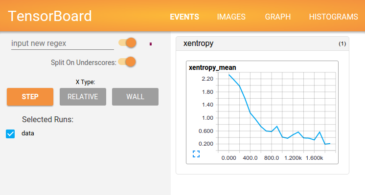
After the training is over (or even in progress!), You can run Tensorboard, specifying the absolute path to the directory with logs:

tensorboard --logdir=/path/to/logs

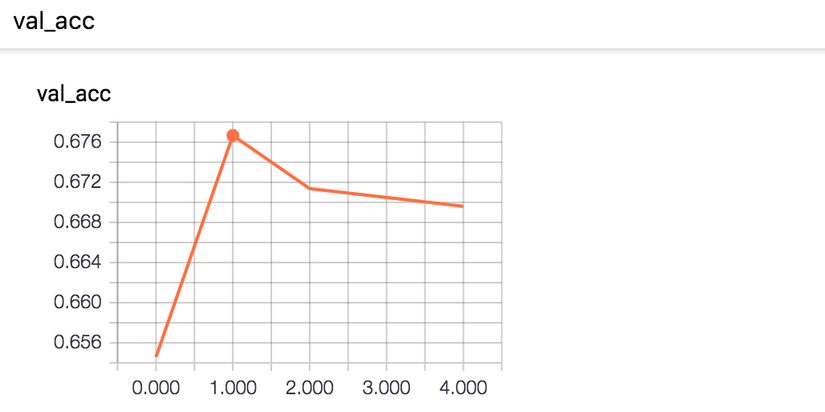
There you can see, for example, how the loss value was changed on the validation sample:

Advanced graphs

Now consider the construction of a slightly more complex calculation graph. A neural network can have a lot of inputs and outputs, input data can be transformed by a variety of mappings. To reuse parts of complex graphs (in particular, for transfer learning), it makes sense to describe a model in a modular style that allows you to easily extract, save, and apply to the new input data pieces of the model.

It is most convenient to describe the model by mixing both the Functional API and the Sequential API described in the previous article.

Consider this approach using the Siamese Network model as an example. Similar models are actively used in practice to obtain vector representations that have useful properties. For example, a similar model can be used to learn such a display of faces photos into a vector, that vectors for similar faces will be close to each other. In particular, this is used by image search applications, such as FindFace.

An illustration of the model Siamese can be seen on the diagram:

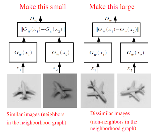
Here the function G transforms the input image into a vector, after which the distance between the vectors for a pair of pictures is calculated. If pictures from the same class, the distance should be minimized, if from different - to maximize. After such a neural network is trained, we can represent an arbitrary picture as a vector G(x) and use this representation either to search for the nearest images, or as a vector of attributes for other machine learning algorithms. Let's describe the model in the code accordingly, making it as easy as possible to extract and reuse the parts of the neural network. First, we define on Keras a function that maps the input vector:

def create_base_network(input_dim):
    seq = Sequential()
    seq.add(Dense(128, input_shape=(input_dim,), activation='relu'))
    seq.add(Dropout(0.1))
    seq.add(Dense(128, activation='relu'))
    seq.add(Dropout(0.1))
    seq.add(Dense(128, activation='relu'))
    return seq

Note: we described the model using the Sequential API, but wrapped it in a function. Now we can create such model by calling this function, and apply it using the Functional API to the input data:

base_network = create_base_network(input_dim)

input_a = Input(shape=(input_dim,))
input_b = Input(shape=(input_dim,))

processed_a = base_network(input_a)
processed_b = base_network(input_b)

Now, the processed_a and processed_b variables are the vector representations obtained by applying the network defined earlier to the input data. You need to calculate the distance between them. To do this, Keras provides a wrapper function Lambda, which represents any expression as a Layer. Do not forget that we process data in batches, so that all tensors always have an extra dimension, which is responsible for the size of the batch.

from keras import backend as K

def euclidean_distance(vects):
    x, y = vects
    return K.sqrt(K.sum(K.square(x - y), axis=1, keepdims=True))

distance = Lambda(euclidean_distance)([processed_a, processed_b])

Great, we got the distance between internal representations, now it remains to assemble inputs and distance into one model.

model = Model([input_a, input_b], distance)

Thanks to the modular structure, we can use base_network separately, which is especially useful after learning the model. How can this be done? Let's look at the layers of our model:

>>> model.layers
[<keras.engine.topology.InputLayer object at 0x7f238fdacb38>, <keras.engine.topology.InputLayer object at 0x7f238fdc34a8>, <keras.models.Sequential object at 0x7f239127c3c8>, <keras.layers.core.Lambda object at 0x7f238fddc4a8>]

We see the third object in the list of type models.Sequential. This is the model that maps the input image to a vector. To extract it and use it as a full-fledged model (it is possible to learn, validate, embed in another graph), it is enough just to pull it out from the list of layers:

>>> embedding_model = model.layers[2]
>>> embedding_model.layers
[<keras.layers.core.Dense object at 0x7f23c4e557f0>, <keras.layers.core.Dropout object at 0x7f238fe97908>, <keras.layers.core.Dense object at 0x7f238fe44898>, <keras.layers.core.Dropout object at 0x7f238fe449e8>, <keras.layers.core.Dense object at 0x7f238fe01f60>]

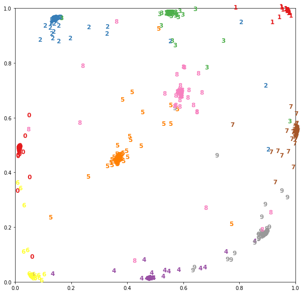
For example, for a Siamese network already trained on MNIST data with a dimension at the base_model output of two, you can visualize the vector representations as follows: Load the data and give the picture size 28x28 to the flat vectors.

(x_train, y_train), (x_test, y_test) = mnist.load_data()
x_test = x_test.reshape(10000, 784)

We will display the images using the previously extracted model:

embeddings = embedding_model.predict(x_test)

Now in embeddings two-dimensional vectors are written, they can be represented on a plane: A full example of the Siamese network can be seen here.

Conclusion

It's time to discuss the pros and cons of Keras. The obvious advantages are the simplicity of creating models, which translates into high speed prototyping. In general, this framework is becoming more and more popular:

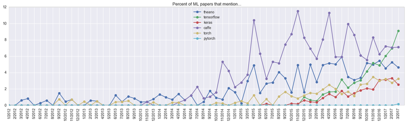
Keras over the year caught up with Torch, which has been developing for 5 years, judging by the mentions in scientific articles. It seems that his goal - ease of use - François Chollet (François Chollet, author of Keras) has achieved. Moreover, his initiative did not go unnoticed: after just a few months of development, Google invited him to do it in the team developing Tensorflow. And also with the version of Tensorflow 1.2 Keras will be included in the TF (tf.keras).

Also I must say a few words about the shortcomings. Unfortunately, Keras's idea of code universality is not always fulfilled: Keras 2.0 broke compatibility with the first version, some functions began to be called differently, some moved, in general, the story is similar to the second and third python. The difference is that in the case of Keras, only the second version was chosen for development. Also, Keras code runs on Tensorflow while slower than on Theano (although for native code the frameworks are at least comparable).

Thank you for attention. See you soon