Libraries for deep learning: Keras [Part 1]
Bài đăng này đã không được cập nhật trong 4 năm
Libraries for deep learning: Keras

Initially, Keras grew like a convenient superstructure over Theano. Hence his Greek name - κέρας, which means "horn" in Greek, which, in turn, is a reference to the Odyssey of Homer. Although, since then, a lot of water has flowed, and Keras began to support Tensorflow first, and then became a part of it. However, our story will be devoted not to the difficult fate of this framework, but to its capabilities.
Installation
To work with Keras, you should already have at least one of the frameworks installed - Theano or Tensorflow. Installation of Keras is extremely simple, because it is the usual Python package:
pip install keras
Now we can begin to parse it, but first we'll talk about backends.
Backends
Backends - this is what made Keras famous and popular (among other advantages, which we will discuss below). Keras allows you to use various other frameworks as a backend. In this case, the code written by you will be executed regardless of the backend used. Development began, as we said, with Theano, but over time Tensorflow was added. Now Keras works by default with it, but if you want to use Theano, then there are two options for doing it:
- Edit the configuration file keras.json, which lies under the path
$HOME/.keras/keras.json(or%USERPROFILE%\.keras\keras.jsonfor Windows operating systems). We need a fieldbackend:
{
"image_data_format": "channels_last",
"epsilon": 1e-07,
"floatx": "float32",
"backend": "theano"
}
- The second way is to set the environment variable
KERAS_BACKEND, for example, like this:
KERAS_BACKEND=theano python -c "from keras import backend"
Using Theano backend.
There is also the MXNet Keras backend, which does not yet have all the functionality, but if you use MXNet, you can pay attention to this possibility. There is also an interesting project Keras.js, which makes it possible to run the trained Keras models from the browser on machines where there is a GPU.
Practical example
Data
 The learning of any model in machine learning begins with the data. Keras contains several training datasets inside, but they are already in a convenient form and do not allow to show the full power of Keras. Therefore, we will take a more crude dataset. This will be a dataset of 20 newsgroups - 20 thousand news messages from Usenet groups, roughly equally distributed among 20 categories. We will teach our network to correctly distribute messages on these newsgroups.
from sklearn.datasets import fetch_20newsgroups
newsgroups_train = fetch_20newsgroups(subset='train')
newsgroups_test = fetch_20newsgroups(subset='test')
Preprocessing
Keras contains tools for easy preprocessing of texts, pictures and time series, in other words, the most common types of data. Today we work with texts, so we need to break them into tokens and bring them to the matrix form.
tokenizer = Tokenizer(num_words=max_words)
tokenizer.fit_on_texts(newsgroups_train["data"])  # Now Tokenizer knows the dictionary for this body of texts

x_train = tokenizer.texts_to_matrix(newsgroups_train["data"], mode='binary')
x_test = tokenizer.texts_to_matrix(newsgroups_test["data"], mode='binary')
At the output, we have obtained binary matrices of these sizes:
x_train shape: (11314, 1000)
x_test shape: (7532, 1000)
The first number is the number of documents in the sample, and the second is the size of our dictionary (one thousand in this example).
We also need to convert the class labels to the matrix form for learning by cross-entropy. To do this, we translate the class number into a so-called one-hot vector, i.e. a vector consisting of zeros and one unit:
y_train = keras.utils.to_categorical(newsgroups_train["target"], num_classes)
y_test = keras.utils.to_categorical(newsgroups_test["target"], num_classes)
At the output, we also obtain binary matrices of these sizes:
y_train shape: (11314, 20)
y_test shape: (7532, 20)
As we can see, the sizes of these matrices partially coincide with the data matrices (the first coordinate - the number of documents in the training and test samples), and partially - no. On the second coordinate, we have the number of classes (20, as the name of the data set indicates).
All, now we are ready to teach our network to classify the news!
Model
The model in Keras can be described in two main ways:
Sequential API
The first is a consistent description of the model, for example, like this:
model = Sequential()
model.add(Dense(512, input_shape=(max_words,)))
model.add(Activation('relu'))
model.add(Dropout(0.5))
model.add(Dense(num_classes))
model.add(Activation('softmax'))
or like this:
model = Sequential([
    Dense(512, input_shape=(max_words,)),
    Activation('relu'),
    Dropout(0.5),
    Dense(num_classes),
    Activation('softmax')
])
Functional API
There is no fundamental difference between the methods, choose which one you prefer.
The Model class (and Sequential inherited from it) has a user-friendly interface that allows you to see which layers are included in the model - model.layers, inputs - model.inputs, and outputs - model.outputs.
Also a very convenient method of displaying and saving the model is model.to_yaml.
This is the config for our model.
backend: tensorflow
class_name: Model
config:
  input_layers:
  - [input_4, 0, 0]
  layers:
  - class_name: InputLayer
    config:
      batch_input_shape: !!python/tuple [null, 1000]
      dtype: float32
      name: input_4
      sparse: false
    inbound_nodes: []
    name: input_4
  - class_name: Dense
    config:
      activation: linear
      activity_regularizer: null
      bias_constraint: null
      bias_initializer:
        class_name: Zeros
        config: {}
      bias_regularizer: null
      kernel_constraint: null
      kernel_initializer:
        class_name: VarianceScaling
        config: {distribution: uniform, mode: fan_avg, scale: 1.0, seed: null}
      kernel_regularizer: null
      name: dense_10
      trainable: true
      units: 512
      use_bias: true
    inbound_nodes:
    - - - input_4
        - 0
        - 0
        - {}
    name: dense_10
  - class_name: Activation
    config: {activation: relu, name: activation_9, trainable: true}
    inbound_nodes:
    - - - dense_10
        - 0
        - 0
        - {}
    name: activation_9
  - class_name: Dropout
    config: {name: dropout_5, rate: 0.5, trainable: true}
    inbound_nodes:
    - - - activation_9
        - 0
        - 0
        - {}
    name: dropout_5
  - class_name: Dense
    config:
      activation: linear
      activity_regularizer: null
      bias_constraint: null
      bias_initializer:
        class_name: Zeros
        config: {}
      bias_regularizer: null
      kernel_constraint: null
      kernel_initializer:
        class_name: VarianceScaling
        config: {distribution: uniform, mode: fan_avg, scale: 1.0, seed: null}
      kernel_regularizer: null
      name: dense_11
      trainable: true
      units: !!python/object/apply:numpy.core.multiarray.scalar
      - !!python/object/apply:numpy.dtype
        args: [i8, 0, 1]
        state: !!python/tuple [3, <, null, null, null, -1, -1, 0]
      - !!binary |
        FAAAAAAAAAA=
      use_bias: true
    inbound_nodes:
    - - - dropout_5
        - 0
        - 0
        - {}
    name: dense_11
  - class_name: Activation
    config: {activation: softmax, name: activation_10, trainable: true}
    inbound_nodes:
    - - - dense_11
        - 0
        - 0
        - {}
    name: activation_10
  name: model_1
  output_layers:
  - [activation_10, 0, 0]
keras_version: 2.0.4
This allows you to save models in a human-readable form, and also instantiate models from this description:
from keras.models import model_from_yaml

yaml_string = model.to_yaml()
model = model_from_yaml(yaml_string)
It is important to note that the model saved in text form (by the way, it is possible to save it also in JSON) does not contain weights. For saving and loading of weights using save_weights function and load_weights respectively.
Visualization of the model
You can not ignore visualization. Keras has built-in visualization for models:
from keras.utils import plot_model
plot_model(model, to_file='model.png', show_shapes=True)
This code will store the following picture under the name model.png:
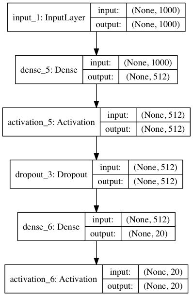
Here we additionally displayed the size of the inputs and outputs for the layers. None, going first in the tuple of sizes is the batch dimension. Because There is None, then the batch can be arbitrary.
If you want to display it in a Jupyter notebook, you need a slightly different code:
from IPython.display import SVG
from keras.utils.vis_utils import model_to_dot

SVG(model_to_dot(model, show_shapes=True).create(prog='dot', format='svg'))
It is important to note that for visualization you need the package graphviz, as well as the python package pydot. There is a subtle point that for the correct operation of the visualization package pydot from the repository will not work, you need to take its updated version of pydot-ng.
pip install pydot-ng
The package graphviz in Ubuntu is set this way (in other Linux distributions it is similar):
apt install graphviz
On MacOS (using the HomeBrew package system):
brew install graphviz
Instructions for installing on Windows can be found here.
Preparing the model for work
So, we have formed our model. Now you need to prepare it for work:
model.compile(loss='categorical_crossentropy',
              optimizer='adam',
              metrics=['accuracy'])
What do the parameters of the compile function mean?
loss is a function of error, in our case it is cross entropy, it was for it that we prepared our labels in the form of matrices;
optimizer - the optimizer used, there could be an ordinary stochastic gradient descent, but Adam shows better convergence on this task;
metrics - the metrics on which the quality of the model is considered, in our case - is the accuracy, that is, the proportion of correctly guessed answers.
Custom loss
Although Keras contains most of the popular error functions, your task may require something unique. To make your own loss, you need a little: just define a function that takes the vectors of correct and predicted answers and issues one number to the output. For training, let's do our own function of calculating the cross-entropy. To make it different, we introduce the so-called clipping - clipping of the vector values from above and below. Yes, another important point: the non-standard loss may need to be described in terms of the underlying framework, but we can do with the tools of Keras.
from keras import backend as K

epsilon = 1.0e-9
def custom_objective(y_true, y_pred):
    '''Yet another cross-entropy'''
    y_pred = K.clip(y_pred, epsilon, 1.0 - epsilon)
    y_pred /= K.sum(y_pred, axis=-1, keepdims=True)
    cce = categorical_crossentropy(y_pred, y_true)
    return cce
Here y_true and y_pred are tensors from Tensorflow, so Tensorflow functions are used for their processing.
To use another loss function, it is enough to change the values of the loss parameter of the compile function, passing there the object of our loss function (in the python function these are also objects, although this is another story altogether):
model.compile(loss=custom_objective,
              optimizer='adam',
              metrics=['accuracy'])
Training and testing
Finally, it's time to learn the model:
history = model.fit(x_train, y_train,
                    batch_size=batch_size,
                    epochs=epochs,
                    verbose=1,
                    validation_split=0.1)
fit method does just that. It takes the input sample along with the x_train and y_train tags, the size of the batch - batch_size , which limits the number of examples submitted at a time, the number of epochs for learning epochs (one epoch is the once complete model-driven training sample) what percentage of the training sample should be given for validation - validation_split.
This method returns history is a history of errors at each step of the learning process.
And finally, testing. Method evaluate receives a test sample along with its labels for the input. The metric was set even during the preparation for work, so that nothing else is needed. (But we will also specify the size of the batch).
score = model.evaluate(x_test, y_test, batch_size=batch_size)
Callbacks
It is also necessary to say a few words about the important features of Keras, like callbacks. Through them a lot of useful functionality is implemented. For example, if you train the network for a very long time, you need to understand when it's time to stop, if the error on your dataset has ceased to decrease. The described functionality is called early stopping. Let's see how we can apply it in training our network:
from keras.callbacks import EarlyStopping
early_stopping=EarlyStopping(monitor='value_loss')

history = model.fit(x_train, y_train,
                    batch_size=batch_size,
                    epochs=epochs,
                    verbose=1,
                    validation_split=0.1,
                    callbacks=[early_stopping])
Do an experiment and check how early stopping works in our example.
Conclusion
That's it, we made the first models on Keras! We hope that gives them an opportunity you are interested in, so you will use it in their work. In general, I can recommend Keras to use when you need to quickly compose and test the network for a specific task. But if you need some complicated things, like a non-standard layer or parallelizing the code to several GPUs, then it's better (and sometimes just inevitable) to use the underlying framework Tensorflow.
Also, I highly recommend that you familiarize yourself with the official examples, on which this article is based. In the next article, we will continue to explore the possibilities of Tensorflow for visualizing various data in the training of our models.
Thank you for your attention and I wish you every success in the deep machine learning.
All rights reserved
