Paper reading | Video Swin Transformer

Đóng góp của bài báo

Kiến trúc Transformer ngày càng chiếm sóng trên mọi mặt trận cụ thể trong các bài toán liên quan tới lĩnh vực Computer Vision. Bài báo được giới thiệu dưới đây đề xuất một kiến trúc backbone thuần transformer cho bài toán video recognition. Mô hình được đề xuất được dựa trên mô hình nổi tiếng là Swin Transformer được tinh chỉnh để sử dụng cho Video có tên là Video Swin Transformer. Vì model đề xuất được tinh chỉnh từ Swin Transformer nên nó có thể tận dụng pretrained trên các bộ dataset hình ảnh lớn. Với model được pretrain trên ImageNet-21K, nhóm tác giả nhận thấy rằng learning rate của kiến trúc backbone cần có giá trị nhỏ hơn so với phần head của kiến trúc (được khởi tạo ngẫu nhiên). Kết quả là backbone sẽ "quên" các tham số được pretrained và dữ liệu chậm hơn trong khi vẫn fit với video input mới, dẫn đến khả năng tổng quát hóa tốt hơn. Model đạt kết quả khả quan trên các bộ dữ liệu video hành động như Kinetics.

Phương pháp

Kiến trúc tổng quan

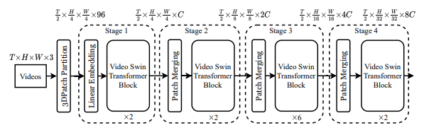
Trên hình là kiến trúc tổng quan của Video Swin Transformer (ở phiên bản Tiny). Input video có kích thước là $T \times H \times W \times 3$ trong đó có $T$ frame và mỗi frame gồm $H \times W \times 3$ pixel. Nếu như trong model ViT, ta chia ảnh thành các patch (2D) thì trong Video Swin Transformer, ta cũng chia video thành các patch (3D) có kích thước là $2 \times 4 \times 4 times 3$ , các patch này còn được gọi là các token. Khi đó, với input video được định nghĩa ban đầu, đi qua 3D patch partitioning layer ta sẽ có $\frac{T}{2} \times \frac{H}{4} \times \frac{W}{4}$ 3D token, mỗi token bao gồm một feature 96 chiều. Tiếp theo, ta sử dụng một linear embedding layer để chiếu các feature của mỗi token về số chiều tùy ý, kí hiệu là $C$ . Ý tưởng được thể hiện trong code như sau:

class PatchEmbed3D(nn.Module):
    """ Video to Patch Embedding.
    Args:
        patch_size (int): Patch token size. Default: (2,4,4).
        in_chans (int): Number of input video channels. Default: 3.
        embed_dim (int): Number of linear projection output channels. Default: 96.
        norm_layer (nn.Module, optional): Normalization layer. Default: None
    """
    def __init__(self, patch_size=(2,4,4), in_chans=3, embed_dim=96, norm_layer=None):
        super().__init__()
        self.patch_size = patch_size

        self.in_chans = in_chans
        self.embed_dim = embed_dim

        self.proj = nn.Conv3d(in_chans, embed_dim, kernel_size=patch_size, stride=patch_size)
        if norm_layer is not None:
            self.norm = norm_layer(embed_dim)
        else:
            self.norm = None

    def forward(self, x):
        """Forward function."""
        # padding
        _, _, D, H, W = x.size()
        if W % self.patch_size[2] != 0:
            x = F.pad(x, (0, self.patch_size[2] - W % self.patch_size[2]))
        if H % self.patch_size[1] != 0:
            x = F.pad(x, (0, 0, 0, self.patch_size[1] - H % self.patch_size[1]))
        if D % self.patch_size[0] != 0:
            x = F.pad(x, (0, 0, 0, 0, 0, self.patch_size[0] - D % self.patch_size[0]))

        x = self.proj(x)  # B C D Wh Ww
        if self.norm is not None:
            D, Wh, Ww = x.size(2), x.size(3), x.size(4)
            x = x.flatten(2).transpose(1, 2)
            x = self.norm(x)
            x = x.transpose(1, 2).view(-1, self.embed_dim, D, Wh, Ww)

        return x

Nhìn kiến trúc tổng quan trong ảnh trên, ta sẽ thấy là model không downsample temporal dimension (luôn duy trì là $\frac{T}{2}$ ) và thực hiện downsample spatial 2 lần tại patch merging layer tại mỗi stage. Patch merging layer sẽ thực hiện concat các feature của $2 \times 2$ patch lân cận (theo spatial) và sau đó sử dụng linear layer để chiếu các concat feature xuống còn một nửa số chiều. Ví dụ, linear layer trong stage thứ 2 chiếu concat $4C$ chiều cho mỗi token xuống còn $2C$ chiều.

Ta có thể đọc đoạn code module PatchMerging sau để hiểu rõ hơn ý tưởng:

class PatchMerging(nn.Module):
    """ Patch Merging Layer
    Args:
        dim (int): Number of input channels.
        norm_layer (nn.Module, optional): Normalization layer.  Default: nn.LayerNorm
    """
    def __init__(self, dim, norm_layer=nn.LayerNorm):
        super().__init__()
        self.dim = dim
        self.reduction = nn.Linear(4 * dim, 2 * dim, bias=False)
        self.norm = norm_layer(4 * dim)

    def forward(self, x):
        """ Forward function.
        Args:
            x: Input feature, tensor size (B, D, H, W, C).
        """
        B, D, H, W, C = x.shape

        # padding
        pad_input = (H % 2 == 1) or (W % 2 == 1)
        if pad_input:
            x = F.pad(x, (0, 0, 0, W % 2, 0, H % 2))

        x0 = x[:, :, 0::2, 0::2, :]  # B D H/2 W/2 C
        x1 = x[:, :, 1::2, 0::2, :]  # B D H/2 W/2 C
        x2 = x[:, :, 0::2, 1::2, :]  # B D H/2 W/2 C
        x3 = x[:, :, 1::2, 1::2, :]  # B D H/2 W/2 C
        x = torch.cat([x0, x1, x2, x3], -1)  # B D H/2 W/2 4*C

        x = self.norm(x)
        x = self.reduction(x)

        return x

Thành phần chính của kiến trúc là Video Swin Transformer block được xây dựng bằng cách thay module multi-head self-attention (MSA) trong Transformer layer thành module 3D shifted window based multi-head self-attention và giữ nguyên các thành phần khác.

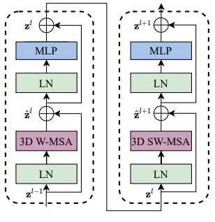
Cụ thể, Video Transformer block gồm một module 3D shifted window base MSA và tiếp đến là feed-forward network (FFN). Feed-forward network bao gồm 2 layer MLP và GELU activation ở giữa. Layer normalization (LN) được sử dụng trước mỗi MSA module và FFN, một kết nối tắt được sử dụng sau mỗi module.

3D Shifted Window based MSA Module

Vì video có số lượng input token lớn hơn rất nhiều so với ảnh do có thêm chiều temporal ( $T$ ), nếu sử dụng self-attention toàn cục có thể dẫn tới chi phí tính toán và bộ nhớ rất lớn. Do đó, nhóm tác giả giới thiệu một inductive bias cục bộ cho module self-attention và được chứng minh là hiệu quả cho bài toán video recognition.

Multi-head self-attention trên non-overlapping 3D windows Từ cơ chế MSA cho từng non-overlapping 2D window sử dụng trong bài toán image recognition, nhóm tác giả mở rộng ý tưởng này cho đầu vào là video. Cho một video gồm $T' \times H' \times W'$ 3D token và một 3D window có kích thước $P \times M \times M$ . Ta thực hiện chia các input token thành $\left\lceil\frac{T^{\prime}}{P}\right\rceil \times\left\lceil\frac{H^{\prime}}{M}\right\rceil \times\left\lceil\frac{W^{\prime}}{M}\right\rceil$ non-overlapping 3D window.

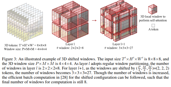
Ví dụ trong hình trên, một input size có $8 \times 8 \times 8$ token và một window size có $4 \times 4 \times 4$ , số lượng window trong layer $l$ sẽ là $2 \times 2 \times 2 = 8$ . Sau đó, MSA sẽ được thực hiện trên mỗi 3D window này.

3D Shifted Windows Vì MSA được áp dụng cho từng 3D window riêng lẻ, điều này làm mất đi sự kết nối giữa các window khác nhau và do đó làm hạn chế khả năng biểu diễn của mô hình. Vì vậy, nhóm tác giả mở rộng cơ chế shifted 2d window của Swin Transformer thành 3D window với mục tiêu capture được những liên kết giữa các window trong khi vẫn duy trì được chi phí tính toán tối ưu của non-overlapping window based self-attention.

Cụ thể, cho số lượng input 3D token là $T' \times H' \times W'$ và một 3D window có kích thước $P \times M \times M$ , với 2 layer liên tiếp, self-attention module trong layer đầu sử dụng chiến lược chia window sao cho nhận được $\left\lceil\frac{T^{\prime}}{P}\right\rceil \times\left\lceil\frac{H^{\prime}}{M}\right\rceil \times\left\lceil\frac{W^{\prime}}{M}\right\rceil$ non-overlapping 3D windows. Với module self-attention ở layer thứ 2, chiến lược chia window là ta sẽ di chuyển window theo trục temporal, height và width với step là $\left(\frac{P}{2}, \frac{M}{2}, \frac{M}{2}\right)$ .

Với cách tiếp cận trên, 2 Video Swin Transformer block liên tiếp được tính như sau:

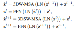
trong đó $\hat{\mathbf{z}}^l$ và mathbf{z}}^l lần lượt là các feature của 3D(S)W-MSA module và FFN module trong block $l$ ; 3DW-MSA và 3DSW-MSA lần lượt là 3D window based multi-head self-attention using regular và shifted window partitioning configurations.

3D Relative Position Bias Các nghiên cứu trước đó chỉ ra rằng sử dụng relative position bias cho mỗi head trong tính toán self-attention đem lại một số lợi ích. Trong bài báo, nhóm tác giả giới thiệu 3D relative position bias $B \in \mathbb{R}^{P^2 \times M^2 \times M^2}$ cho mỗi head như sau:

trong đó $Q, K, V \in \mathbb{R}^{P M^2 \times d}$ là các ma trận query, key và value. $d$ là chiều của các feature query và key. $PM^2$ là số lượng token trong 3D window. Vì vị trí tương đối theo mỗi trục nằm trong đoạn $[-P + 1, P - 1]$ (temporal) hoặc $[-M + 1, M - 1]$ (height hoặc width), nhóm tác giả thực hiện tam số hóa ma trận bias có kích thước nhỏ hơn $\hat{B} \in \mathbb{R}^{(2 P-1) \times(2 M-1) \times(2 M-1)}$ và giá trị $B$ được lấy từ $\hat{B}$ .

Cuối cùng, code cho module 3D window attention sẽ như sau:

def window_partition(x, window_size):
    """
    Args:
        x: (B, D, H, W, C)
        window_size (tuple[int]): window size
    Returns:
        windows: (B*num_windows, window_size*window_size, C)
    """
    B, D, H, W, C = x.shape
    x = x.view(B, D // window_size[0], window_size[0], H // window_size[1], window_size[1], W // window_size[2], window_size[2], C)
    windows = x.permute(0, 1, 3, 5, 2, 4, 6, 7).contiguous().view(-1, reduce(mul, window_size), C)
    return windows


def window_reverse(windows, window_size, B, D, H, W):
    """
    Args:
        windows: (B*num_windows, window_size, window_size, C)
        window_size (tuple[int]): Window size
        H (int): Height of image
        W (int): Width of image
    Returns:
        x: (B, D, H, W, C)
    """
    x = windows.view(B, D // window_size[0], H // window_size[1], W // window_size[2], window_size[0], window_size[1], window_size[2], -1)
    x = x.permute(0, 1, 4, 2, 5, 3, 6, 7).contiguous().view(B, D, H, W, -1)
    return x


def get_window_size(x_size, window_size, shift_size=None):
    use_window_size = list(window_size)
    if shift_size is not None:
        use_shift_size = list(shift_size)
    for i in range(len(x_size)):
        if x_size[i] <= window_size[i]:
            use_window_size[i] = x_size[i]
            if shift_size is not None:
                use_shift_size[i] = 0

    if shift_size is None:
        return tuple(use_window_size)
    else:
        return tuple(use_window_size), tuple(use_shift_size)


class WindowAttention3D(nn.Module):
    """ Window based multi-head self attention (W-MSA) module with relative position bias.
    It supports both of shifted and non-shifted window.
    Args:
        dim (int): Number of input channels.
        window_size (tuple[int]): The temporal length, height and width of the window.
        num_heads (int): Number of attention heads.
        qkv_bias (bool, optional):  If True, add a learnable bias to query, key, value. Default: True
        qk_scale (float | None, optional): Override default qk scale of head_dim ** -0.5 if set
        attn_drop (float, optional): Dropout ratio of attention weight. Default: 0.0
        proj_drop (float, optional): Dropout ratio of output. Default: 0.0
    """

    def __init__(self, dim, window_size, num_heads, qkv_bias=False, qk_scale=None, attn_drop=0., proj_drop=0.):

        super().__init__()
        self.dim = dim
        self.window_size = window_size  # Wd, Wh, Ww
        self.num_heads = num_heads
        head_dim = dim // num_heads
        self.scale = qk_scale or head_dim ** -0.5

        # define a parameter table of relative position bias
        self.relative_position_bias_table = nn.Parameter(
            torch.zeros((2 * window_size[0] - 1) * (2 * window_size[1] - 1) * (2 * window_size[2] - 1), num_heads))  # 2*Wd-1 * 2*Wh-1 * 2*Ww-1, nH

        # get pair-wise relative position index for each token inside the window
        coords_d = torch.arange(self.window_size[0])
        coords_h = torch.arange(self.window_size[1])
        coords_w = torch.arange(self.window_size[2])
        coords = torch.stack(torch.meshgrid(coords_d, coords_h, coords_w))  # 3, Wd, Wh, Ww
        coords_flatten = torch.flatten(coords, 1)  # 3, Wd*Wh*Ww
        relative_coords = coords_flatten[:, :, None] - coords_flatten[:, None, :]  # 3, Wd*Wh*Ww, Wd*Wh*Ww
        relative_coords = relative_coords.permute(1, 2, 0).contiguous()  # Wd*Wh*Ww, Wd*Wh*Ww, 3
        relative_coords[:, :, 0] += self.window_size[0] - 1  # shift to start from 0
        relative_coords[:, :, 1] += self.window_size[1] - 1
        relative_coords[:, :, 2] += self.window_size[2] - 1

        relative_coords[:, :, 0] *= (2 * self.window_size[1] - 1) * (2 * self.window_size[2] - 1)
        relative_coords[:, :, 1] *= (2 * self.window_size[2] - 1)
        relative_position_index = relative_coords.sum(-1)  # Wd*Wh*Ww, Wd*Wh*Ww
        self.register_buffer("relative_position_index", relative_position_index)

        self.qkv = nn.Linear(dim, dim * 3, bias=qkv_bias)
        self.attn_drop = nn.Dropout(attn_drop)
        self.proj = nn.Linear(dim, dim)
        self.proj_drop = nn.Dropout(proj_drop)

        trunc_normal_(self.relative_position_bias_table, std=.02)
        self.softmax = nn.Softmax(dim=-1)

    def forward(self, x, mask=None):
        """ Forward function.
        Args:
            x: input features with shape of (num_windows*B, N, C)
            mask: (0/-inf) mask with shape of (num_windows, N, N) or None
        """
        B_, N, C = x.shape
        qkv = self.qkv(x).reshape(B_, N, 3, self.num_heads, C // self.num_heads).permute(2, 0, 3, 1, 4)
        q, k, v = qkv[0], qkv[1], qkv[2]  # B_, nH, N, C

        q = q * self.scale
        attn = q @ k.transpose(-2, -1)

        relative_position_bias = self.relative_position_bias_table[self.relative_position_index[:N, :N].reshape(-1)].reshape(
            N, N, -1)  # Wd*Wh*Ww,Wd*Wh*Ww,nH
        relative_position_bias = relative_position_bias.permute(2, 0, 1).contiguous()  # nH, Wd*Wh*Ww, Wd*Wh*Ww
        attn = attn + relative_position_bias.unsqueeze(0) # B_, nH, N, N

        if mask is not None:
            nW = mask.shape[0]
            attn = attn.view(B_ // nW, nW, self.num_heads, N, N) + mask.unsqueeze(1).unsqueeze(0)
            attn = attn.view(-1, self.num_heads, N, N)
            attn = self.softmax(attn)
        else:
            attn = self.softmax(attn)

        attn = self.attn_drop(attn)

        x = (attn @ v).transpose(1, 2).reshape(B_, N, C)
        x = self.proj(x)
        x = self.proj_drop(x)
        return x

Một số biến thể của kiến trúc mô hình

Nhóm tác giả giới thiệu 4 phiên bản của Video Swin Transformer. Ta có 2 tham số chính cho các phiên bản khác nhau là $C$ và số layer.

Swin-T: $C$ = 96, layer numbers = {2, 2, 6, 2}
Swin-S: $C$ = 96, layer numbers ={2, 2, 18, 2}
Swin-B: $C$ = 128, layer numbers ={2, 2, 18, 2}
Swin-L: $C$ = 192, layer numbers ={2, 2, 18, 2}

trong đó $C$ là số channel của các hidden layer trong stage đầu tiên. Window size được đặt mặc định là $P = 8$ và $M = 7$ . Số chiều query của mỗi head là $d = 32$ và expansion layer cho mỗi MLP được đặt là $\alpha = 4$ .

Khởi tạo từ Pretrained Model

Vì model Video Swin Transformer được "cải tiến" từ Swin Transformer, model Video Swin Transformer có thể khởi tạo từ pretrained trên bộ dữ liệu lớn của Swin Transformer. So sánh với Swin Transformer chỉ có 2 block trong Video Swin Transformer là có shape khác, đó là linear embedding layer trong stage đầu tiên và relative position bias trong Video Swin Transformer block.

Vì trong model Video Swin Transformer, input token được thêm chiều temporal có giá trị là 2, điều này làm cho shape của linear embedding layer thành $96 \times C$ so với $48 \times C$ của Swin Transformer. Để tận dụng được weight pretrain của Swin, nhóm tác giả thực hiện duplicate weight lên 2 lần và nhân toàn bộ ma trận với 0.5 để giữ cho mean và variance của output không đổi. Shape của relative position bias matrix là $(2P - 1, 2M - 1, 2M - 1)$ so với $(2M −1, 2M −1)$ trong Swin. Để làm cho relative position bias giống nhau giữa mỗi frame, nhóm tác giả duplicate ma trận trong pretrained model $2P - 1$ lần để đạt được shape $(2P − 1, 2M − 1, 2M − 1)$ .

Thực nghiệm

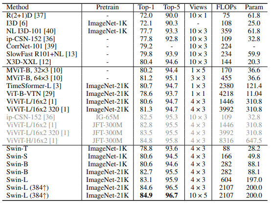
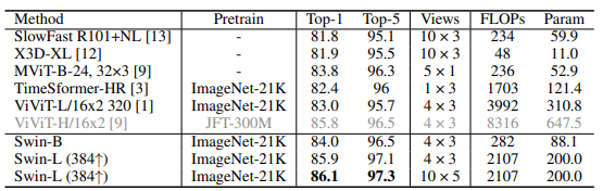
Hai bảng dưới đây là so sánh kết quả SOTA trên Kinetic-400.

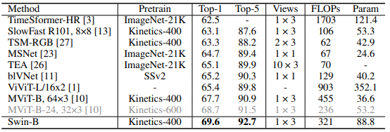
Bảng dưới là so sánh kết quả SOTA trên tập Something-Something v2.

Kết luận

Vậy là qua bài báo bạn đã có thêm một lựa chọn model để thực nghiệm cho bài toán Video Recognition. Bài báo cung cấp kiến trúc thuần Transformer và đạt các kết quả ấn tượng trên 3 tập dữ liệu benchmark cho Video Recognition Kinetics-400, Kinetics-600 và Something-Something v2.