Anomaly Detection of Time Series Data Using Machine Learning & Deep Learning
Bài đăng này đã không được cập nhật trong 4 năm
Introduction to Time Series Data
Time Series is defined as a set of observations taken at a particular period of time. For example, having a set of login details at regular interval of time of each user can be categorized as a time series. On the other hand, when the data is collected at once or irregularly, it is not taken as a time series data.
Time series data can be classified into two types -
Stock Series - It is a measure of attributes at a particular point in time and taken as a stock takes.
Flow Series - It is a measure of activity at a specific interval of time. It contains effects related to the calendar.
Time series is a sequence that is taken successively at the equally pace of time. It appears naturally in many application areas such as economics, science, environment, medicine, etc. There are many practical real life problems where data might be correlated with each other and are observed sequentially at the equal period of time. This is because, if the repeatedly observe the data at a regular interval of time, it is obvious that data would be correlated with each other.
With the use of time series, it becomes possible to imagine what will happen in the future as future event depends upon the current situation. It is useful to divide the time series into historical and validation period. The model is built to make predictions on the basis of historical data and then this model is applied to the validation set of observations. With this process, the idea is developed how the model will perform in forecasting.
Time Series is also known as the stochastic process as it represents the vector of stochastic variables observed at regular interval of time.
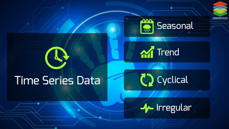
Components of Time Series Data
In order to analyze the time series data, there is a need to understand the underlying pattern of data ordered at a particular time. This pattern is composed of different components which collectively yield the set of observations of time series.
The Components of time series data are given below -
- Trend
- Cyclical
- Seasonal
- Irregular
Trend - It is a long pattern present in the time series. It produces irregular effects and can be positive, negative, linear or nonlinear. It represents the variations of low frequency and the high and medium frequency of data is filtered out from the time series.
If the time series does not contain any increasing or decreasing pattern, then time series is taken as stationary in the mean.
There are two types of the trend -
Deterministic - In this case, the effects of the shocks present in the time series are eliminated i.e. revert to the trend in long run.
Stochastic - It is the process in which the effects of shocks are never eliminated as they have permanently changed the level of the time series.
The stochastic process having a stationarity around the deterministic process is known as trend stationary process.
Cyclic - The pattern exhibit up and down movements around a specified trend is known as cyclic pattern. It is a kind of oscillations present in the time series. The duration of cyclic pattern depends upon the industries and business problems to be analysed. This is because the oscillations are dependable upon the business cycle.
They are larger variations that are repeated in a systematic way over time. The period of time is not fixed and usually composed of at least 2 months in duration. The cyclic pattern is represented by a well-shaped curve and shows contraction and expansion of data.
Seasonal - It is a pattern that reflects regular fluctuations. These short-term movements occur due to the seasonal factors and custom factors of people. In this case, the data faces regular and predictable changes that occurred at regular intervals of calendar. It always consist of fixed and known period.
The main sources of seasonality are given below -
- Climate
- Institutions
- Social habits and practices
- Calendar
How is the seasonal component estimated?
If the deterministic analysis is performed, then the seasonality will remain same for similar interval of time. Therefore, it can easily be modelled by dummy variables. On the other hand, this concept is not fulfilled by stochastic analysis. So, dummy variables are not appropriate because the seasonal component changes throughout the time series.
Different models to create a seasonal component in time series are given below -
Additive Model - It is the model in which the seasonal component is added with the trend component.
Multiplicative Model - In this model seasonal component is multiplied with the intercept if trend component is not present in the time series. But, if time series have trend component, sum of intercept and trend is multiplied with the seasonal component.
Irregular - It is an unpredictable component of time series. This component cannot be explained by any other component of time series because these variational fluctuations are known as random component. When the trend cycle and seasonal component is removed, it becomes residual time series. These are short term fluctuations that are not systematic in nature and have unclear patterns.
Difference between Time Series Data and Cross-Section Data
Time Series Data is composed of collection of data of one specific variable at particular interval of time. On the other hand, Cross-Section Data is consist of collection of data on multiple variables from different sources at a particular interval of time.
Collection of company’s stock market data at regular interval of year is an example of time series data. But when the collection of company’s sales revenue, sales volume is collected for the past 3 months then it is taken as an example of cross-section data.
Time series data is mainly used for obtaining results over an extended period of time but, cross-section data focuses on the information received from surveys at a particular time.
What is Time Series Analysis?
Performing analysis of time series data is known as Time Series Analysis. Analysis is performed in order to understand the structure and functions produced by the time series. By understanding the mechanism of time series data a mathematical model could easily be developed so that further predictions, monitoring and control can be performed.
Two approaches are used for analyzing time series data are -
- In the time domain
- In the frequency domain
Time series analysis is mainly used for -
- Decomposing the time series
- Identifying and modeling the time-based dependencies
- Forecasting
- Identifying and model the system variation
Need of Time Series Analysis
In order to model successfully, the time series is important in machine learning and deep learning. Time series analysis is used to understand the internal structure and functions that are used for producing the observations. Time Series analysis is used for -
Descriptive - In this case, patterns are identified in correlated data. In other words, the variations in trends and seasonality in the time series are identified.
Explanation - In this understanding and modeling of data is performed.
Forecasting - Here, the prediction from previous observations is performed for short term trends.
Invention Analysis - In this case, effect performed by any event in time series data is analyzed.
Quality Control - When the specific size deviates it provides an alert.
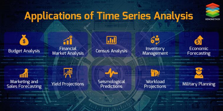
Applications of Time Series Analysis
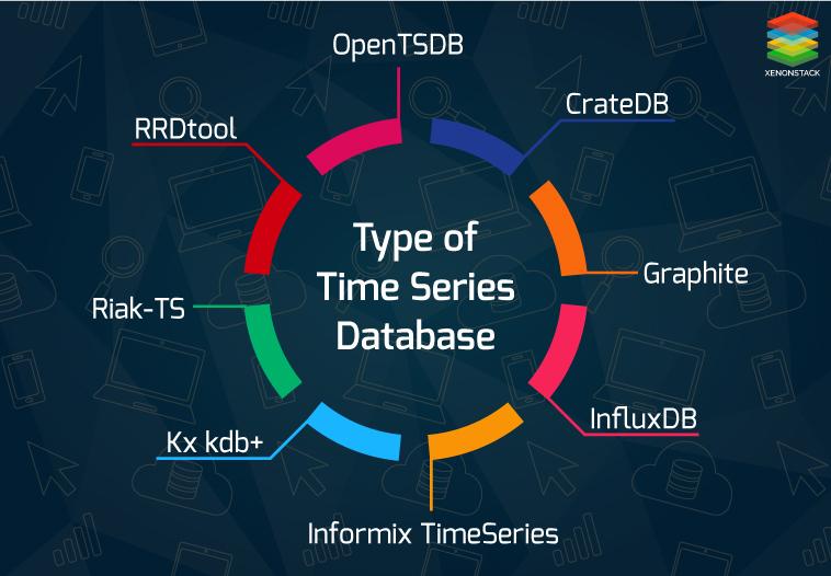
Time Series Database and its types
Time series database is a software which is used for handling the time series data. Highly complex data such higher transactional data is not feasible for the relational database management system. Many relational systems does not work properly for time series data. Therefore, time series databases are optimised for the time series data. Various time series databases are given below -
- CrateDB
- Graphite
- InfluxDB
- Informix TimeSeries
- Kx kdb+
- Riak-TS
- RRDtool
- OpenTSDB
What is Anomaly?
Anomaly is defined as something that deviates from the normal behaviour or what is expected. For more clarity let’s take an example of bank transaction. Suppose you have a saving bank account and you mostly withdraw Rs 10,000 but, one day Rs 6,00,000 amount is withdrawn from your account. This is unusual activity for bank as mostly, Rs 10,000 is deducted from the account. This transaction is an anomaly for bank employees.
The anomaly is a kind of contradictory observation in the data. It gives the proof that certain model or assumption does not fit into the problem statement.
Different Types of Anomalies
Different types of anomalies are given below -
Point Anomalies - If the specific value within the dataset is anomalous with respect to the complete data then it is known as Point Anomalies. The above mentioned example of bank transaction is an example of point anomalies.
Contextual Anomalies - If the occurrence of data is anomalous for specific circumstances, then it is known as Contextual Anomalies. For example, the anomaly occurs at a specific interval of period.
Collective Anomalies - If the collection of occurrence of data is anomalous with respect to the rest of dataset then it is known as Collective Anomalies. For example, breaking the trend observed in ECG.
Models of Time Series Data
ARIMA Model - ARIMA stands for Autoregressive Integrated Moving Average. Auto Regressive (AR) refers as lags of the differenced series, Moving Average (MA) is lags of errors and I represents the number of difference used to make the time series stationary.
Assumptions followed while implementing ARIMA Model are as under -
Time series data should posses stationary property: this means that the data should be independent of time. Time series consist of cyclic behaviour and white noise is also taken as a stationary.
ARIMA model is used for a single variable. The process is meant for regression with the past values.
In order to remove non-stationarity from the time series data the steps given below are followed -
Find the difference between the consecutive observations.
For stabilizing the variance log or square root of the time series data is computed.
If the time series consists of the trend, then the residual from the fitted curve is modulated.
ARIMA model is used for predicting the future values by taking the linear combination of past values and past errors. The ARIMA models are used for modeling time series having random walk processes and characteristics such as trend, seasonal and nonseasonal time series.
Holt-Winters - It is a model which is used for forecasting the short term period. It is usually applied to achieve exponential smoothing using additive and multiplicative models along with increasing or decreasing trends and seasonality. Smoothing is measured by beta and gamma parameters in the holt’s method.
When the beta parameter is set to FALSE, the function performs exponential smoothing.
The gamma parameter is used for the seasonal component. If the gamma parameter is set to FALSE, a non-seasonal model is fitted.
How to find Anomaly in Time Series Data
AnomalyDetection R package -
It is a robust open source package used to find anomalies in the presence of seasonality and trend. This package is build on Generalised E-Test and uses Seasonal Hybrid ESD (S-H-ESD) algorithm. S-H-ESD is used to find both local and global anomalies. This package is also used to detect anomalies present in a vector of numerical variables. Is also provides better visualization such that the user can specify the direction of anomalies.
Principal Component Analysis -
It is a statistical technique used to reduce higher dimensional data into lower dimensional data without any loss of information. Therefore, this technique can be used for developing the model of anomaly detection. This technique is useful at that time of situation when sufficient samples are difficult to obtain. So, PCA is used in which model is trained using available features to obtain a normal class and then distance metrics is used to determine the anomalies.
Chisq Square distribution -
It is a kind of statistical distribution that constitutes 0 as minimum value and no bound for the maximum value. Chisq square test is implemented for detecting outliers from univariate variables. It detects both lowest and highest values due to the presence of outliers on both side of the data.
What are Breakouts in Time Series Data?
Breakout are significant changes observed in the time series data. It consist of two characteristics that are given below -
Mean shift - It is defined as a sudden change in time series. For example the usage of CPU is increased from 35% to 70%. This is taken as a mean shift. It is added when the time series move from one steady state to another state.
Ramp Up - It is defined as a sudden increase in the value of the metric from one steady state to another. It is a slow process as compared with the mean shift. It is a slow transition process from one stable state to another.
In Time series often more than one breakouts are observed.
How to detect Breakouts in Time Series Data?
In order to detect breakouts in time series Twitter has introduced a package known as BreakoutDetection package. It is an open source package for detecting breakouts at a fast speed. This package uses E-Divisive with Medians (EDM) algorithm to detect the divergence within the mean. It can also be used to detect the change in distribution within the time series.
Need of Machine Learning and Deep Learning in Time Series Data
Machine learning techniques are more effective as compared with the statistical techniques. This is because machine learning have two important features such as feature engineering and prediction. The feature engineering aspect is used to address the trend and seasonality issues of time series data. The issues of fitting the model to time series data can also be resolved by it.
Deep Learning is used to combine the feature extraction of time series with the non-linear autoregressive model for higher level prediction. It is used to extract the useful information from the features automatically without using any human effort or complex statistical techniques.
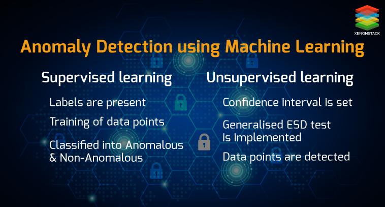
Anomaly Detection using Machine Learning
There are two most effective techniques of machine learning such as supervised and unsupervised learning.
Firstly, supervised learning is performed for training data points so that they can be classified into anomalous and non-anomalous data points. But, for supervised learning, there should be labeled anomalous data points.
Another approach for detecting anomaly is unsupervised learning. One can apply unsupervised learning to train CART so that prediction of next data points in the series could be made. To implement this, confidence interval or prediction error is made. Therefore, to detect anomalous data points Generalised ESD-Test is implemented to check which data points are present within or outside the confidence interval
The most common supervised learning algorithms are supervised neural networks, support vector machine learning, k-nearest neighbors, Bayesian networks and Decision trees.
In the case of k-nearest neighbors, the approximate distance between the data points is calculated and then the assignment of unlabeled data points is made according to the class of k-nearest neighbor.
On the other hand, Bayesian networks can encode the probabilistic relationships between the variables. This algorithm is mostly used with the combination of statistical techniques.
The most common unsupervised algorithms are self-organizing maps (SOM), K-means, C-means, expectation-maximization meta-algorithm (EM), adaptive resonance theory (ART), and one-class support vector machine.
Anomaly Detection using Deep Learning
Recurrent neural network is one of the deep learning algorithm for detecting anomalous data points within the time series. It consist of input layer, hidden layer and output layer. The nodes within hidden layer are responsible for handling internal state and memory. They both will be updated as the new input is fed into the network. The internal state of RNN is used to process the sequence of inputs. The important feature of memory is that it can automatically learns the time-dependent features.
The process followed by RNN is described below -
Continue Reading The Full Article At - XenonStack.com/Blog
All rights reserved
