I. Giới thiệu về AdaBoost

Các model Machine learning (không sử dụng Neural Network) có thể khái quát như sau:

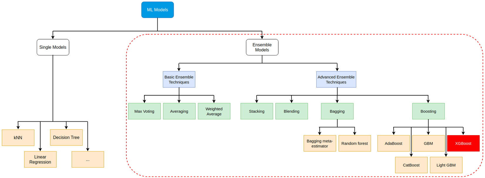
Để hiểu rõ hơn các bạn có thể tham khảo 2 bài viết Gradient Boosting - Tất tần tật về thuật toán mạnh mẽ nhất trong Machine Learning và Ensemble learning và các biến thể (P1)

Trong bài viết này, mình giới thiệu 1 thuật toán, có thể coi là tổ tiên khai sinh ra Gradient Boosting hiện tại - AdaBoost (Hiện giờ AdaBoost được coi là 1 trường hợp đặc biệt của Gradient Boosting)

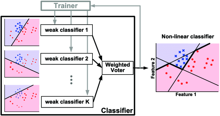
AdaBoost, tên đầy đủ là Adaptive Boosting, là thuật toán thuộc nhánh Boosting trong Ensemble learning. Với ý tưởng đơn giản là sử dụng các cây quyết định (1 gốc, 2 lá) để đánh trọng số cho các điểm dữ liệu, từ đó tối thiểu hóa trọng số các điểm bị phân loại sai (trọng số lớn), để tăng hiệu suất của mô hình

II. Giải thuật AdaBoost

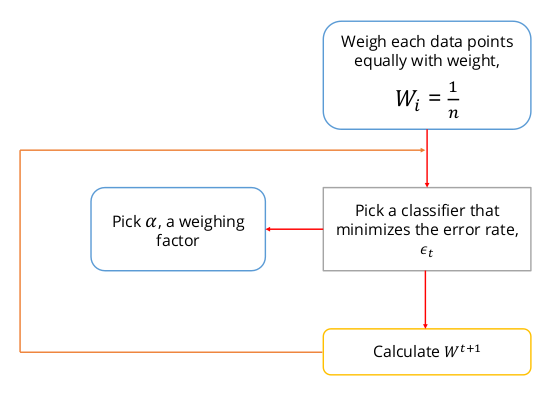
AdaBoost có thể hình dung đơn giản qua flowchart:

Có nghĩa là, với:

• Tập dữ liệu $\{(x_1, y_1), (x_2, y_2),..., (x_n, y_n)\}$, với $y_i \in \{-1, 1\}, i \in \{1, 2, ..., n\}$
• Trọng số các điểm dữ liệu tại weak leaner thứ t: $w_1^t, w_2^t,..., w_n^t, i \in \{1, 2, ..., n\}$
• weak-learners $h: x\rightarrow\{-1, 1\}$
• Error function: $E(f(x), y, i) = e^{-y_i f(x_i)}$, trong đó $f(x_i) = \alpha h(x_i)$
• Output: $H_t(x)$, $H_t(x)$ còn được gọi là strong leaner tại thời điểm t

Các bước triển khai cho thuật toán được mô tả như sau:

B1: Khởi tạo weights cho từng input: $w_{i}^{1} = \frac{1}{n}, i \in \{1, 2, ..., n\} \rightarrow \sum_{i}{w_i^{1}} = 1$

B2: Với mỗi vòng lặp $t \in \{1, 2,..., T\}$:

• Tìm weak-learners $h_{t} (x)$ để tối thiểu hóa tổng error của các điểm bị phân loại sai, $E = \sum_{y_i \# h_t(x_i)}{w_i^t}$
• Tỉ lệ lỗi của weak leaners: $\varepsilon_{t} = \frac{\sum_{y_i \# h_t(x_i)}{w_i^t}}{\sum_{i=1}^{n}{w_{i}^t}} = \sum_{y_i \# h_t(x_i)}{w_i^t}$, vì $\sum_{i=1}^{n}{w_{i}^t} = 1$
• Gán trọng số cho weak-learners giá trị $\alpha_{t} = \frac{1}{2}\ln(\frac{1-\varepsilon_t}{\varepsilon_t})$
• Cập nhật strong learner: $H_{t}(x) = H_{t-1}(x) + \alpha_{t}h_t(x)$
• Cập nhật lại weights:
  • $w_{i}^{t+1} = w_{i}^{t} e^{- y_i \alpha_t h_t(x_i)}, i \in \{1, 2, ..., n\}$
  • Chuẩn hóa lại weights: $w_i^{t+1} \leftarrow \frac{w_i^{t+1}}{\sum_{i}{w_i^{t+1}}}$, có nghĩa là $\sum_{i}{w_i^{t+1}} = 1$

B3: Ouput chính là dấu của biểu thức tổng các weak-learners nhân với trọng số của chúng, hay

$$H(x) = sign(\sum_{t=1}^T{\alpha_t h_t(x)})$$

Vậy, câu hỏi được đặt ra là

Tại sao gán trọng số $\alpha_t = \frac{1}{2}ln(\frac{1 - \varepsilon_{t}}{\varepsilon_{t}})$ cho weak-learners?

Việc đặt lại trọng số cho các weak-learners là vô cùng quan trọng, ở đây, thuật toán đã chỉ ra rằng khi $\alpha_{t} = \frac{1}{2}\ln(\frac{1-\varepsilon_t}{\varepsilon_t})$, chúng ta có thể tối thiểu hóa hàm loss $L_{exp} = e^{-yh(x)}$ trong quá trình training.

Như thuật toán ở trên, sau vòng lặp thứ $(t-1)$, strong leaner là tổ hợp tuyến tính của các weak leaners dưới dạng biểu thức:

$$H_{t-1}(x_i) = \alpha_1h_1(x_i) + \alpha_2h_2(x_i) + ... + \alpha_{t-1}h_{t-1}(x_i)$$

Class của điểm $x_i$ chính là dấu của biểu thức $H_{t}(x_i)$. Tại vòng lặp $t$, để tăng độ chính xác cho $H(x)$, ta cộng thêm weak-learners $h_t$ nhân với trọng số $\alpha_t$ của nó:

$$H_{t}(x_i) = H_{t-1}(x_i) + \alpha_{t}h_t(x_i)$$

Gọi $E$ là tổng exponential loss của $H_t$ trên từng điểm dữ liệu, ta có

$$E = \sum_{i=1}^{N}{e^{-y_i H_t(x_i)}}$$

$$= \sum_{i=1}^{N}{e^{-y_i (H_{t-1}(x_i) + \alpha_{t}h_t(x_i))}}$$

$$= \sum_{i=1}^{N}{e^{-y_i H_{t-1}(x_i)}e^{-y_i \alpha_t h_t(x_i)}}$$

Đặt trọng số $w_i^1$ = $\frac{1}{n}$ và $w_i^t = e^{-y_i H_{t-1}(x_i)}$ với t > 1, ta được:

$$E = \sum_{i=1}^{N}{w_i^te^{-y_i \alpha_t h_t(x_i)}}$$

Nhận thấy có 2 khả năng xảy ra với mỗi điểm trong tập dữ liệu:

• Phân loại đúng: $y_i = h_t(x_i)$
• Phân loại sai: $y_i$ # $h_t(x_i)$

Khi đó:

$$E = \sum_{y_i = h_t(x_i)}{w_i^te^{-\alpha_t}} + \sum_{y_i \# h_t(x_i)}{w_i^te^{\alpha_t}}$$

Đến đây chỉ cần sử dụng kiến thức đạo hàm lớp 12 để tối thiểu hóa loss $E$ theo $\alpha_t$, như sau:

$$\frac{\delta E}{\delta \alpha_t} = \frac{\delta(\sum_{y_i = h_t(x_i)}{w_i^te^{-\alpha_t}} + \sum_{y_i \# h_t(x_i)}{w_i^te^{\alpha_t}})}{\delta \alpha_t}$$

Min xảy ra khi $\frac{\delta E}{\delta \alpha_t} = 0$, hay

$$-\sum_{y_i = h_t(x_i)}{w_i^te^{-\alpha_t}} + \sum_{y_i \# h_t(x_i)}{w_i^te^{\alpha_t}} = 0$$

Vì $e^{-\alpha_t}$ và $e^{\alpha_t}$ không phụ thuộc vào i, nên:

$$e^{-\alpha_t}\sum_{y_i = h_t(x_i)}{w_i^t} = e^{\alpha_t}\sum_{y_i \# h_t(x_i)}{w_i^t}$$

Lấy Loga Nepe 2 vế,

$$-\alpha_t + ln(\sum_{y_i = h_t(x_i)}{w_i^t}) = \alpha_t + ln(\sum_{y_i \# h_t(x_i)}{w_i^t})$$

Chuyển vế,

$$-2\alpha_t = ln(\sum_{y_i \# h_t(x_i)}{w_i^t}) - ln(\sum_{y_i = h_t(x_i)}{w_i^t})$$

Áp dụng $lna - lnb = ln\frac{a}{b}$,

$$-2\alpha_t = ln(\frac{\sum_{y_i \# h_t(x_i)}{w_i^t}}{ \sum_{y_i = h_t(x_i)}{w_i^t}})$$

$$\alpha_t = \frac{1}{2}ln(\frac{\sum_{y_i = h_t(x_i)}{w_i^t}}{ \sum_{y_i \# h_t(x_i)}{w_i^t}})$$

Vì tỉ lệ lỗi của weak leaners $\varepsilon_{t} = \sum_{y_i \# h_t(x_i)}{w_i^t} / \sum_{i=1}^{n}{w_{i}^t}$ và $\sum_{y_i = h_t(x_i)}{w_i^t} + \sum_{y_i \# h_t(x_i)}{w_i^t} = \sum_{i=1}^{n}{w_{i}^t}$ nên,

$$\alpha_t = \frac{1}{2}ln(\frac{\sum_{i=1}^{n}{w_{i}^t} - \sum_{y_i \# h_t(x_i)}{w_i^t}}{ \sum_{y_i \# h_t(x_i)}{w_i^t}})$$

$$\alpha_t = \frac{1}{2}ln(\frac{1}{\varepsilon_{t}} - 1)$$

$$\alpha_t = \frac{1}{2}ln(\frac{1 - \varepsilon_{t}}{\varepsilon_{t}})$$

Trên đây là cách mà giá trị $\alpha$ được tìm ra, cũng khá dễ để chứng minh. Lý thuyết về AdaBoost vậy đủ rồi, cùng mình đến với code nào (Lý thuyết cũng chỉ là lý thuyết )

II. Implement model

2.1 Các thư viện cần dùng

import numpy as np
import matplotlib.pyplot as plt
import matplotlib as mpl
from typing import Optional

from sklearn.tree import DecisionTreeClassifier
from sklearn.ensemble import AdaBoostClassifier

from sklearn.metrics import confusion_matrix, accuracy_score, f1_score, recall_score
from sklearn.metrics import classification_report, log_loss

import warnings
warnings.filterwarnings('ignore')

2.2 Xây dựng model

Vì $y$ nhận 2 giá trị -1 và 1, nên mình cần có 1 hàm kiểm tra gíá trị của $y$

def check(y):
    assert set(y) == {-1,1}
    return y

Bảng dưới đây giải thích các biến mình sử dụng trong code mà ý nghĩa của chúng:

Tên biến	Chiều	Kí hiệu trong giải thuật	Ý nghĩa
sample_weights	(T,n)	w	Ma trận trọng số các điểm trên các weak-learners
current_sew	(n,)	$w_i^t$	Trọng số các điểm tại weak-learners thứ t
new_sew	(n,)	$w_i^{t+1}$	Trọng số các điểm tại weak-learners thứ t+1
stumps	(T,)	h	Danh sách các weak-learners)
stump	(1,)	$h_t$	Weak-learners thứ t
stump_weights	(T,)	A	Trọng số các weak-learners
stump_weight	(1,)	$\alpha_t$	Trọng số weak-learners thứ t
errors	(T,)	E	Danh sách tỉ lệ lỗi của các weak-learners
error	(1,)	$\varepsilon_t$	Tỉ lệ lỗi của weak-learners thứ t
predict(X)	(n,)	$H_t$	Ouput thuật toán

Tiếp theo là xây dựng mô hình

Khởi tạo các biến

def init_model(iters, X):
    n = X.shape[0]
    sample_weights = np.zeros((iters, n))
    stumps = np.zeros(iters, dtype= object)
    stump_weights = np.zeros(iters)
    errors = np.zeros(iters)
    return stumps, stump_weights, sample_weights, errors

Triển khai mô hình

Tóm tắt lại thuật toán:

Tại mỗi vòng lặp, chọn weak-learners $h_t$, tối thiểu hóa tổng trọng số các điểm bị phân loại sai $\sum_{y_i \# h_t(x_i)}{w_i^t}$, sau đấy tính tỉ lệ lỗi $\varepsilon_{t} = \sum_{y_i \# h_t(x_i)}{w_i^t}$, dùng $\varepsilon_{t}$ để tính trọng số cho weak-learners thứ t $\alpha_t = \frac{1}{2}ln(\frac{1 - \varepsilon_{t}}{\varepsilon_{t}})$, cuối cùng dùng kết quả vừa tính được để cải thiện output $H_{t}(x_i) = H_{t-1}(x_i) + \alpha_{t}h_t(x_i)$

Vì mục tiêu bài này là hiểu AdaBoost, nên weak-learners $h_t(x)$ mình sử dụng luôn DecisionTreeClassifier được xây dựng trong sklearn.ensemble với trọng số (max_depth=1, max_leaf_nodes=2)

def AdaBoostClf(X, y, iters= 10):
    n = X.shape[0]
    # Check y
    y = check(y)
    # Initialize
    stumps, stump_weights, sample_weights, errors = init_model(iters= iters, X= X)

    # First weight = 1/n
    sample_weights[0] = np.ones(shape= n) / n

    for i in range(iters):
        # Fit for stump: weak learner
        current_sew = sample_weights[i]
        stump = DecisionTreeClassifier(max_depth= 1, max_leaf_nodes= 2)
        stump = stump.fit(X, y, sample_weight= current_sew)

        # Calculate error
        stump_pred = stump.predict(X)
        error = current_sew[stump_pred != y].sum()
        stump_weight = np.log((1 - error) / error) / 2

        # New sample weight
        new_sew = current_sew * np.exp(-1 * stump_weight * y * stump_pred)

        # Renormalize weights
        new_sew = new_sew / new_sew.sum()

        # If not last iter, update sample weights for i+1
        if (i + 1) < iters:
            sample_weights[i+1] = new_sew

        # Save result
        errors[i] = error
        stumps[i] = stump
        stump_weights[i] = stump_weight

    return stumps, stump_weights, sample_weights

2.3 Predictions

Như đã đề cập ở trên, kết quả phân loại từng điểm chính là dấu của biểu thức

$$H(x) = sign(\sum_{t=1}^T{\alpha_t h_t(x)})$$

với (+) nghĩa là $y(x) = 1$ và (-) là $y(x) = - 1$

def predict(X, stumps, stump_weights):
    stump_preds = np.array([stump.predict(X) for stump in stumps])
    return np.sign(np.dot(stump_weights, stump_preds))

III Testing

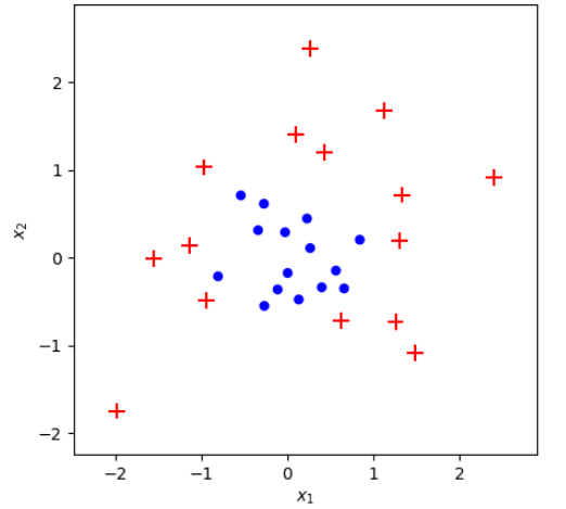
3.1 Fake datasets

Tạo dữ liệu

Mình sử dụng bộ dữ liệu đã đơn giản hóa từ sklearn documentation

def make_dataset(n: int = 100, random_seed: int = None):
    n_per_class = int(n/2)
    if random_seed:
        np.random.seed(random_seed)
    X, y = make_gaussian_quantiles(n_samples=n, n_features=2, n_classes=2)
    return X, y*2-1

X, y = make_dataset(n=30, random_seed=10)

Dữ liệu đã có rồi, tiếp theo mình xây dựng một hàm để biểu diễn các điểm và decision boundary của chúng

def plot_adaboost(X: np.ndarray,
                  y: np.ndarray,
                  stumps= None, stump_weights= None, roll = 0,
                  clf= None,
                  sample_weights: Optional[np.ndarray] = None,
                  ax: Optional[mpl.axes.Axes] = None):

    y = check(y) # Kì vọng nhãn bằng ±1

    if not ax:
        fig, ax = plt.subplots(figsize=(5, 5), dpi=100)
        fig.set_facecolor('white')

    pad = 1
    x_min, x_max = X[:, 0].min() - pad, X[:, 0].max() + pad
    y_min, y_max = X[:, 1].min() - pad, X[:, 1].max() + pad

    if sample_weights is not None:
        sizes = np.array(sample_weights) * X.shape[0] * 100  
    else:
        sizes = np.ones(shape=X.shape[0]) * 100

    X_pos = X[y == 1]
    sizes_pos = sizes[y == 1]
    ax.scatter(*X_pos.T, s=sizes_pos, marker='+', color='red')

    X_neg = X[y == -1]
    sizes_neg = sizes[y == -1]
    ax.scatter(*X_neg.T, s=sizes_neg, marker='.', c='blue')

    if clf:
        plot_step = 0.01
        xx, yy = np.meshgrid(np.arange(x_min, x_max, plot_step),
                             np.arange(y_min, y_max, plot_step))
        Z = clf.predict(np.c_[xx.ravel(), yy.ravel()])
        Z = Z.reshape(xx.shape)

        # If all predictions are positive class, adjust color map acordingly
        if list(np.unique(Z)) == [1]:
            fill_colors = ['r']
        else:
            fill_colors = ['b', 'r']

        ax.contourf(xx, yy, Z, colors=fill_colors, alpha=0.2)

    if roll:
        plot_step = 0.01
        xx, yy = np.meshgrid(np.arange(x_min, x_max, plot_step),
                             np.arange(y_min, y_max, plot_step))

        Z = predict(np.c_[xx.ravel(), yy.ravel()], stumps, stump_weights)
        Z = Z.reshape(xx.shape)

        # If all predictions are positive class, adjust color map acordingly
        if list(np.unique(Z)) == [1]:
            fill_colors = ['r']
        else:
            fill_colors = ['b', 'r']

        ax.contourf(xx, yy, Z, colors=fill_colors, alpha=0.2)

    ax.set_xlim(x_min+0.5, x_max-0.5)
    ax.set_ylim(y_min+0.5, y_max-0.5)
    ax.set_xlabel('$x_1$')
    ax.set_ylabel('$x_2$')

plot_adaboost(X, y)

Performance

Mình sẽ so sánh thử khi train bộ dữ liệu này bằng sklearn.ensemble.AdaBoostClassifier và code tự implement ở trên xem thế nào

clf = AdaBoostClassifier(n_estimators=15, algorithm='SAMME').fit(X, y)
plot_adaboost(X, y, clf=clf)

train_err = (clf.predict(X) != y).mean()
print(f'Train error: {train_err:.1%}')

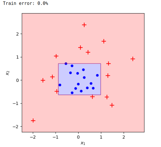
Đơn giản ghê, vậy với code implement thì sao?

# Train with datasets
stumps, stump_weights, sample_weights = AdaBoostClf(X, y, iters= 15)
pred = predict(X, stumps, stump_weights)

# Show metrics
print("Accuracy score: %f" % accuracy_score(y, pred))
print("Confusion Matrix:")
print(confusion_matrix(y, pred))
print(classification_report(y, pred))
print('Log loss:', log_loss(y, pred)/len(y))

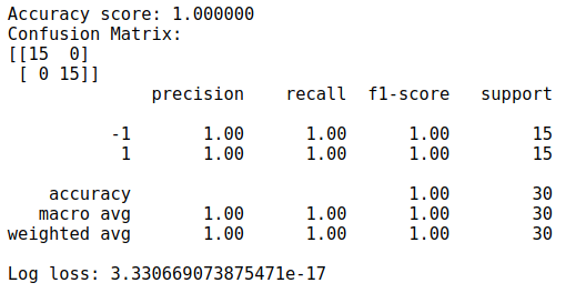
plot_adaboost(X, y, stumps, stump_weights, roll= 1)

Vì bộ dữ liệu khá đơn giản nên kết quả cũng không nằm ngoài dự tính

Visualize kết quả qua từng vòng lặp

Ở trên mình đã lưu toàn bộ kết quả của từng vòng lặp nên bây giờ có thể dùng kết quả đó để visualize cách mà Adaboost hoạt động qua từng vòng lặp đó:

• Độ lớn các điểm trên hình thể hiện trọng số của các điểm, điểm bị phân loại sai trọng số sẽ càng lớn, và ngược lại
• Hình bên trái là weak-learners thứ t
• Hình bên phải thể hiện cho output của AdaBoost sau t weak-learners

def truncate_adaboost(stumps, stump_weights, t: int):
    assert t > 0, 't must be a positive integer'
    x = stumps[:t]
    y = stump_weights[:t]
    return x, y

def plot_staged_adaboost(X, y, stumps, sample_weights, stump_weights, start=0, end=10):
    # larger grid
    fig, axes = plt.subplots(figsize=(8, (end-start)*3),
                             nrows=(end-start),
                             ncols=2,
                             sharex=True,
                             dpi=100)

    fig.set_facecolor('white')
    for i in range(start, end):
        ax1, ax2 = axes[i-start]

        # Plot weak learner
        ehe = ax1.set_title(f'Weak learner at t={i + 1}')
        plot_adaboost(X, y, clf= stumps[i],
                      sample_weights= sample_weights[i],
                      annotate=False, ax=ax1)

        # Plot strong learner
        new_stumps,  new_sw = truncate_adaboost(stumps, stump_weights, t=i + 1)
        ehe = ax2.set_title(f'Strong learner at t={i + 1}')
        plot_adaboost(X, y, new_stumps, new_sw, sample_weights= sample_weights[i], roll=1, annotate=False, ax=ax2)

    plt.tight_layout()
    plt.subplots_adjust(top=0.95)
    plt.show()

Ở dây mình visualize từ cây thứ 10

plot_staged_adaboost(X, y, stumps, sample_weights, stump_weights, start=9, end=15)

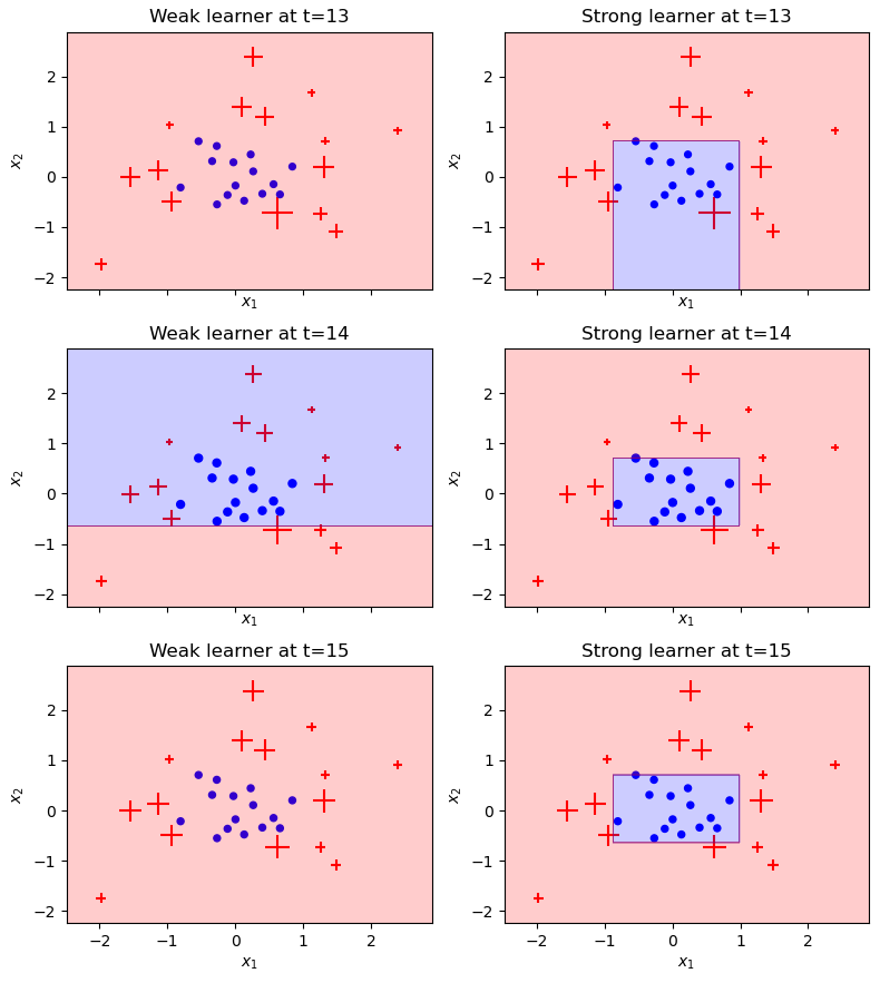
Có thể thấy, tại một số thời điểm (vd: t=11, 13, 15), các điểm được phân loại toàn bộ vào (+), tại sao vậy? Đơn giản là vì với tổng trọng số mẫu hiện tại, cách tốt nhất để tối thiểu hóa trọng số là phân loại tất cả các điểm là (+). Có nghĩa là, vì các mẫu (-) được bao quanh bởi các mẫu (+) có trọng số lớn, nên với 1 cây Decision Tree đơn giản, không thể classify tập dữ liệu bằng 1 đường thẳng phân tách mà làm không làm tăng trọng lượng trong số các diểm (+) bị phân loại sai, điều đó thật tệ với thuật toán, vì khi phân loại tất cả các điểm thành (+), các điểm (-) bị phân loại sai làm tăng trọng số các điểm (-), hay tăng tổng trọng số các điểm lên. Tuy nhiên, điều đó không đủ để ngăn thuật toán hội tụ, với việc cây thứ t phân loại sai làm tăng trọng số các mẫu (-), sẽ giúp cho cây t+1, tìm được 1 đường phân tách mang tính tích cực và quyết định hơn cho thuật toán

3.2 Bộ dữ liệu Titanic

Sau khi đã đại khái biết được sức mạnh của AdaBoost với bộ dữ liệu fake kia rồi, mình muốn chạy thử với bộ dữ liệu thực tế hơn chút xem sao, và lựa chọn của mình là Titanic

Sơ qua về bộ dữ liệu Titanic, là mình phải phân loại xem hành khách là sống(1) hay chết(0) (Feature: Survived) từ những features còn lại. Titanic thì quá là nổi tiếng luôn rồi

Download datasets và tiền xử lý dữ liệu

Mình sẽ xử lý qua chút để dữ liệu clear với mô hình hơn

# Download datasets
titanic = pd.read_csv('https://raw.githubusercontent.com/dhminh1024/practice_datasets/master/titanic.csv')

# Data manipulation
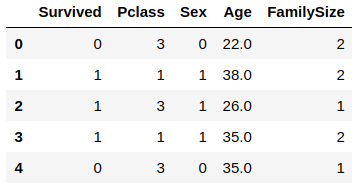
titanic.fillna(titanic['Age'].mean(), inplace=True)
titanic.replace({'Sex':{'male':0, 'female':1}}, inplace=True)
titanic['FamilySize'] = titanic['SibSp'] + titanic['Parch'] + 1
titanic.drop(columns=['PassengerId', 'Name', 'SibSp', 'Parch', 'Ticket', 'Fare', 'Cabin', 'Embarked'], inplace=True)
titanic.head()

Vì giá trị output y là {+1, -1} nên mình đã đổi toàn bộ giá trị 0 thành giá trị -1. Tiếp theo mình chia bộ dữ liệu ra làm 2 phần train và val

from sklearn.model_selection import train_test_split

X = titanic[['Pclass', 'Sex', 'Age', 'FamilySize']].values
y = titanic[['Survived']].values
y[y == 0] = -1    # y must be {+1, -1}

X_train, X_val, y_train, y_val = train_test_split(X, y, test_size=0.2, random_state=102)

print('Training set:', X_train.shape, y_train.shape)
print('Val set:', X_val.shape, y_val.shape)

Sau khi đã có 2 tập dữ liệu, bước tiếp theo là fit với mô hình

# Training
stumps1, stump_weights1, sample_weights1 = AdaBoostClf(X= X_train, y= y_train.reshape(-1), iters= 10)
predt = predict(X_val, stumps1, stump_weights1)

Và đây là kết quả

# Show metrics
print("Accuracy score: %f" % accuracy_score(y_val, predt))
print("Confusion Matrix:")
print(confusion_matrix(y_val, predt))
print(classification_report(y_val, predt))
print('Log loss:', log_loss(y_val, predt)/len(y_val))

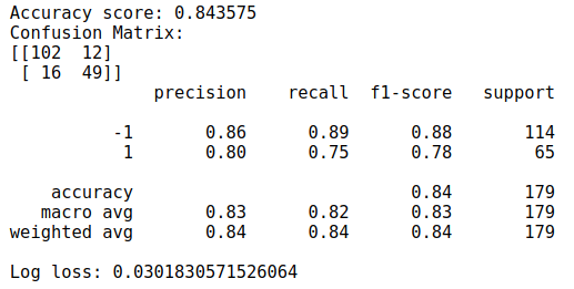
Cũng không tệ, AdaBoost dù không phải top trong Ensemble, nhưng dù sao vẫn là 1 thuật toán vô cùng mạnh mẽ

IV. Lời kết

Vậy là mình đã giới thiệu đến các bạn thuật toán AdaBoost, nếu có thắc mắc, góp ý, hoặc muốn biết thêm về thuật nào khác, hãy comment để mình biết nhé. Cảm ơn các bạn đã dành thời gian đọc bài viết của mình. See ya!! (KxSS)

Tham khảo

1. Data Blog
2. Wikipedia
3. Step by step AdaBoost