First off, let's make some things clear. We, some of the Framgiers of Bangladesh branch, are going to storm Viblo with a series of blogs on machine learning in the upcoming days and here goes the first one by me. You can read some other relevant posts on the same topic here, here and here. I would recommend you to have a quick look on the write-ups following the first two links before you start reading this one. This way time will be saved for you from understanding the basics in detail and me explaining them in this post once again, especially the Linear Regression Model which you can find by clicking the second link. At the same time you might like to take a tour to the very recent news on Google's new AI in the DeepMind project that has learned to become "Highly Aggressive" in stressful situations which has been made possible by a set of highly sophisticated machine learning approaches. Who knows, Logistic Regression could be one of them.

---

The Basics

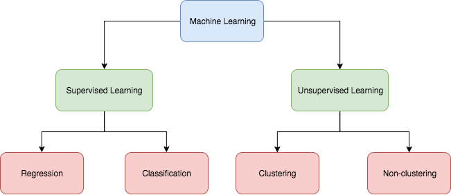
Machine learning can be broadly divided into two types: 1. Supervised learning: we are given a data set and already know what our correct output should look like, having the idea that there is a relationship between the input and the output. Supervised learning can be of two types: i. Regression: we try to predict results within a continuous output, meaning that we are trying to map input variables to some continuous function. For example, given data about the size some houses on the real estate market, we're trying to predict their price. The price of a house can be any number within a huge range from say, $1000 to $1,000,000. So price as a function of size is a continuous output. Therefore, this is a regression problem. ii. Classification: as the type itself indicates, in this type of learning we try to predict results in a discrete output or class. In other words, we are trying to map input variables into discrete categories. For example, suppose we want to classify the houses into categories like cheap, moderate and expensive. In that case price as a function of size is a discrete output. So this is a classification problem. 2. Unsupervised learning: in unsupervised learning we are given a data set to approach problems with little or no idea what our results should look like. We can derive structure from data where we don't necessarily know the effect of the variables. This learning approach can be of two types too: i. Clustering: suppose we have a collection of 1,000,000 different genes and want to automatically group these genes into groups that are somehow similar or related by different variables like lifespan, location, roles etc. Then we can root for a clustering algorithm. ii. Non-clustering: imagine there's a room full of people in a cocktail party and you want to identify individual voices and music from the mesh of sounds around. A non-clustering approach can help you find a structure in this chaotic environment.

The categorization of these approaches is summed up in the following diagram:

So far I've discussed about different approaches to machine learning. Time to come to our main topic - Logistic Regression - which is basically a classification technique of supervised learning. But before that, let's review the linear regression method first, because this too can be applied to our classification approach.

Classification Using Linear Regression

As said earlier, classification allows us to identify a given piece of data as a member of a discrete class. To do this, we have to develop a classifier and train it with a data set with known class labels. Then whenever a piece of data is fed to the classfier whose class is unknown, the classifier is expected to tell us which class that piece of data belongs to. Some real-life example of this type of classification is checking email if it's spam or not, validating an online transaction if it's fraudulent or not, determining if a tumor is malignant or benign based on its size etc. Let's begin with the tumor example.

Suppose we've got a patient with tumor. It can be either malignant or benign as shown below:

Tumor: Malignant or Benign

We can write this in the following way:

y ∈ { 0, 1,...,n }; where 0: "Negative Class" (e.g. benign), 1: "Positive Class" (e.g. malignant), n∈Z

Here, y is the output that denotes the class which the data belongs to.

Just like linear regression, our classifier needs a hypothesis function, hθ(x) where x is a feature of our data, i.e. the size of the tumor. When we encounter with a piece of information about something, the hypothesis function tells us what that thing is, i.e. which class it belongs to. This is the most important part of any classifier.

Now, let's say we have a data set where there are only two classes - '0' and '1'. Between these two, there lies a threshold value 0.5. If we apply the linear regression method on this data set to build our classifier, we will get a hypothesis function hθ(x), which is a linear equation. Remember how a linear equation looks like? Well, the hθ(x) looks like the following:

hθ(x) = θ0 + θ1x

Here θ0 and θ1 have a long story of their own which we will come to very soon. For now, just sit tight and continue reading.

Now, if we want to identify if a tumor is malignant or benign depending on the value of its size x, the hypothesis function hθ(x) will give us an output that can lie i) on the threshold , ii) below the threshold or iii) above the threshold value.

Let the region from the threshold value to its upper limit (which can be infinite) be of class 1 and below the threshold value be of class 0. Then threshold classifier output hθ(x) at threshold 0.5:

y = 1 if hθ(x) ≥ 0.5 y = 0 if hθ(x) < 0.5

Note that, the value of hθ(x) is always greater than or equal to 0 and less than or equal to 1. Mathematically,

0 ≤ hθ(x) ≤ 1

This is the linear regression method of classification. As you can guess, this classifier will not be able to give us a very accurate result. This is when the logistic regression method comes into play.

Logistic Regression

For multivariate regression, the hypothesis function just mentioned earlier can also be written as follows:

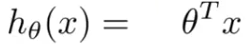
Here, T denotes the transpose of θ vector which can be θ0, θ1,..., θn-1 and x is the feature vector from x0 to xn-1 where x0 = 1. To keep the value of hθ(x) we need to modify the hypothesis function a bit like the following:

hθ(x) = g(z), where z = θ^T*x and g(z) = 1/(1+e^-z)

This is called a Logistic function, hence the name of the classification method. It's also known as Sigmoid function by the way.

So, what does this function tell us about? Let's describe that in mathemetical terms:

hθ(x) = estimated probability that y=1 on input x

Suppose we have a tumor and we know its size. x0 is by default 1 and the tumor size is the x1. If the hypothesis function hθ(x) = 0.7, we can say that the tumor is malignant, assuming that 1 means malignant. In other words the patient has 70% chance that his/her tumor is malignant.

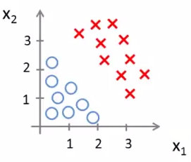
Decision Boundary

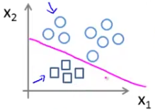
The data set could be scattered like that in the following figure:

In this scenario we need a hypothesis function that will divide the data set into two like that shown below:

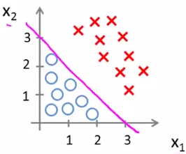
This line, plotted from our hypothesis function, is called the decision boundary. What it means is that the data lying on one side of that line belongs to one class and the data lying on the other side belongs to another.

Suppose, our hypothesis function hθ(x) takes the form of g(θ0 + θ1x1 + θ2x2) where the values of θ0, θ1 and θ2 are -3, 1 and 1 respectively, then our model can be defined as:

Predict "y = 1" if -3 + x1 + x2 ≥ 0 or x1 + x2 ≥ 3 Similarly, predict "y = 0" if x1 + x2 < 3

So, given a piece of data with features x1 and x2 we can predict from our decision boundary which class it belongs to. If x1 + x2 is equal to or greater than 3, then it belongs to class 1, otherwise class 2.

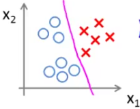
Decision boundary can be non-linear too like the following one:

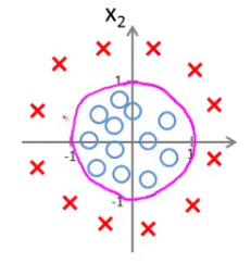
This will lead us to a non-linear decision boundary having a non-linear hypothesis function.

Cost Function

Remember the theta we've dealt with before? Now it's time to tell you their story.

The value(s) of θ in our hypothesis determines how accurate our prediction will be. We have to find out the value(s) of theta(s) in our hypothesis to get the optimum prediction result. And this is where the cost function comes into play.

Cost function gives us a series of output for different values of θ. We will choose the value of θ for which the cost is the absolute minimum. For that value of θ the prediction of our decision boundary will be the most accurate.

The cost function for logistic regression takes the form shown below:

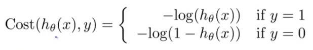
Which can be simplified even more into the following equation:

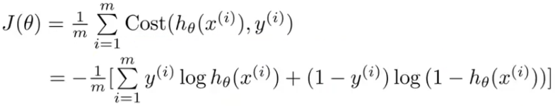
Here, J(θ) is just a fancy way to denote the cost function. The superscript i denotes the ith row of our data set. All we need to do is find the value of θ for which J(θ) is the minimum. How do we do that? Don't worry, there's an algorithm for that too! We call it the Gradient Descent. Here's how it looks like:

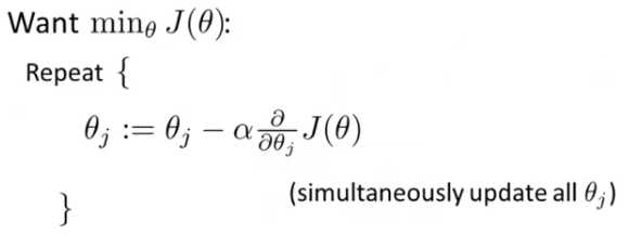
Plugging the value of J(θ) we get:

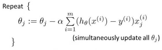
It says that we have to iteratively update the value of all the elements of the θ vector until the partial derivative of the J(θ) is 0 or close to 0.

The value of the constant α is arbitrary, but the results usually get better when the value is small and somewhat between -1 and 1.

Anyway, when we'll reach a point when not a single value in the θ vector is being updated anymore, we settle on those values and those will give us the ultimate hypothesis function, the magical decision boundary!

Multi-class Classification

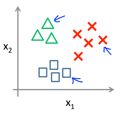
What if there are more than two classes in our data set? For example we want to tag email with 'work', 'friends', 'family' and 'hobby' or the weather to be predicted as 'sunny', 'cloudy', 'rainy' or'snowy'. In these cases we apply the 'One-vs-all' method to our logistic regression model.

If we plot the data set with three classes, it might look like this:

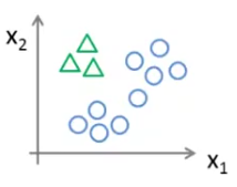
In the 'one-vs-all' method, we first take one class, say A, and separate all the other classes, say B and C, of our training data to group them and treat them as a single class like below:

Then we apply apply our logistic regression model on this data to get the decision boundary between A and all the other classes.

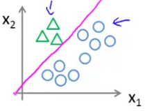
Similarly we can get the decision boundary between B and others and C and others.

Suppose for class A, B and C we get the hypothesis functions h1θ(x), h2θ(x) and h3θ(x) respectively. On a new input of x, we will choose the class for which the value of these three hypothesis function is the maximum. For example, if h2θ(x) > h1θ(x) > h3θ(x) then we'll say the input belongs to class B for some x.

---

That's it! The Logistic Regression model of classification in brief! More on the topic of machine learning is about to come in the upcoming days very soon. So stay tuned to learn more about it.

Until next time, happy learning.