Introduction to Machine Learning

Machine learning is a method of data analysis that automates analytical model building. Using algorithms that iteratively learn from data, machine learning allows computers to find hidden insights without being explicitly programmed where to look. Because of new computing technologies, machine learning today is not like machine learning of the past. It was born from pattern recognition and the theory that computers can learn without being programmed to perform specific tasks; researchers interested in artificial intelligence wanted to see if computers could learn from data. The iterative aspect of machine learning is important because as models are exposed to new data, they are able to independently adapt. They learn from previous computations to produce reliable, repeatable decisions and results. It’s a science that’s not new – but one that’s gaining fresh momentum.

In this post I am going to focus on one of the most oldest and most widely used predictive model in the field of machine learning - Linear regression model for multiple variables assuming that everyone has knowledge about univariate linear variable or linear regression with one variable.

Hypothesis of linear regression

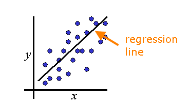
The linear regression model fits a linear function to a set of data points. The form of the hypothesis function is:

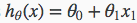
which is equivalent to straight line function y = mx + c. The goal is to minimize the sum of the squared errros to fit a straight line to a set of data points.

We can measure the accuracy of our hypothesis function by using a cost function. This takes an average difference all the results of the hypothesis with inputs from x's and the actual output y's. The cost function for linear regression model is:

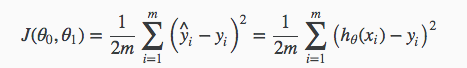
To break it apart, it is 1/2 x‾‾ where x‾‾ is the mean of the squares of hθ(xi)−yi , or the difference between the predicted value (hθ(xi))and the actual value(yi) and m is the number of training examples. This function is otherwise called the "Squared error function", or "Mean squared error". The mean is halved (1/2) as a convenience for the computation of the gradient descent, as the derivative term of the square function will cancel out the 1/2 term.

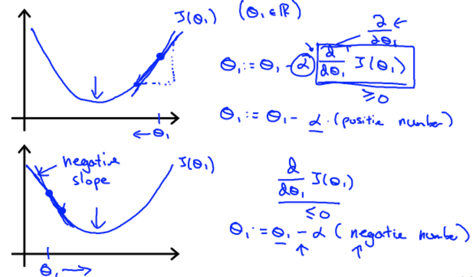
So, the minimum the cost function gets the more accurate, the more data we get, so we have to find the value of θ0 and θ1 such that the cost function is minimum. For determining the vaue of θ0 and θ1 we use gradient descent algorithm. Considering only one feature and θ0=0 we get,

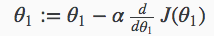
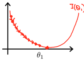
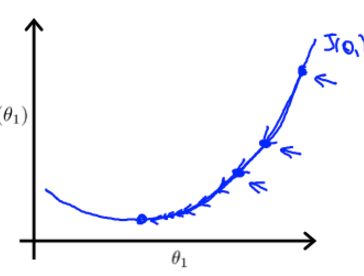
Regardless of the slope's sign for d/dθ1 (J(θ1)), θ1 eventually converges to its minimum value. The following graph shows that when the slope is negative, the value of θ1 increases and when it is positive, the value of θ1 decreases.

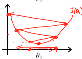
On a side note, we should adjust our parameter α to ensure that the gradient descent algorithm converges in a reasonable time. Failure to converge or too much time to obtain the minimum value imply that our step size is wrong. If α is too small gradient descent can be slow. If α is too large gradient descent can overshoot the minimum, it may fail to converge or may even diverge.

Gradient descent can converge to local minimum even with α learning rate fixed. As we approach to local minimum gradient descent will automatically take smaller steps. So no need to decrease α over time Please check this post https://viblo.asia/sujoy.datta/posts/gAm5yvoqKdb for more detailed explanation on univariate linear regression.

Linear Regression for Multiple variable

Linear regression with multiple variables is also known as "multivariate linear regression". We now introduce notation for equations where we can have any number of input variables. 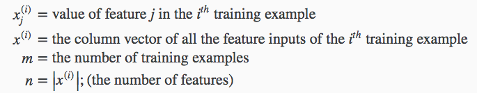The multivariable form of the hypothesis function accommodating these multiple features is as follows:

Using the definition of matrix multiplication, our multivariable hypothesis function can be concisely represented as:

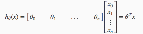This is a vectorization of our hypothesis function for one training example; see the lessons on vectorization to learn more.

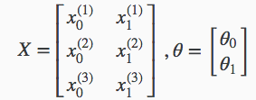
For convenience reasons in this course we assume x(i)0=1 for (i∈1,…,m). This allows us to do matrix operations with theta and x. Hence making the two vectors 'θ' and x(i) match each other element-wise (that is, have the same number of elements: n+1).]

The training examples are stored in X row-wise. The following example shows us the reason behind setting x(i)0=1 : As a result, you can calculate the hypothesis as a column vector of size (m x 1) with:

                                                   hθ(X)=Xθ

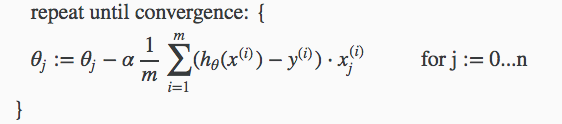
The gradient descent equation itself is generally the same form; we just have to repeat it for our 'n' features:

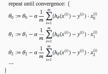
In other words:

We can speed up gradient descent by having each of our input values in roughly the same range. This is because θ will descend quickly on small ranges and slowly on large ranges, and so will oscillate inefficiently down to the optimum when the variables are very uneven.

The way to prevent this is to modify the ranges of our input variables so that they are all roughly the same. Ideally:

      −1 ≤ x(i) ≤ 1

             or

      −0.5 ≤ x(i) ≤ 0.5

These aren't exact requirements; we are only trying to speed things up. The goal is to get all input variables into roughly one of these ranges, give or take a few.

Two techniques to help with this are feature scaling and mean normalization. Feature scaling involves dividing the input values by the range (i.e. the maximum value minus the minimum value) of the input variable, resulting in a new range of just 1. Mean normalization involves subtracting the average value for an input variable from the values for that input variable resulting in a new average value for the input variable of just zero. To implement both of these techniques, adjust your input values as shown in this formula:

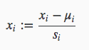Where μi is the average of all the values for feature (i) and si is the range of values (max - min), or si is the standard deviation.

Note that dividing by the range, or dividing by the standard deviation, give different results. For example, if xi represents housing prices with a range of 100 to 2000 and a mean value of 1000, then, xi:=(price−1000)/1900.

Debugging gradient descent Make a plot with number of iterations on the x-axis. Now plot the cost function, J(θ) over the number of iterations of gradient descent. If J(θ) ever increases, then you probably need to decrease α.

Automatic convergence test Declare convergence if J(θ) decreases by less than E in one iteration, where E is some small value such as 10−3. However in practice it's difficult to choose this threshold value.

It has been proven that if learning rate α is sufficiently small, then J(θ) will decrease on every iteration. To summarize:

If α is too small: slow convergence. If α is too large: may not decrease on every iteration and thus may not converge.

Features and Polynomial Regression

We can improve our features and the form of our hypothesis function in a couple different ways.

We can combine multiple features into one. For example, we can combine x1 and x2 into a new feature x3 by taking x1⋅x2.

Polynomial Regression

Our hypothesis function need not be linear (a straight line) if that does not fit the data well.

We can change the behavior or curve of our hypothesis function by making it a quadratic, cubic or square root function (or any other form).

For example, if our hypothesis function is then we can create additional features based on x1, to get the quadratic function 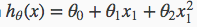or the cubic function 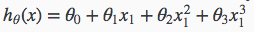In the cubic version, we have created new features x2 and x3 where x2=x21 and x3=x31.

To make it a square root function, we could do: 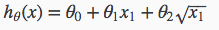One important thing to keep in mind is, if you choose your features this way then feature scaling becomes very important.

Normal Equation

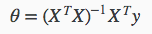
Gradient descent gives one way of minimizing J. Let’s discuss a second way of doing so, this time performing the minimization explicitly and without resorting to an iterative algorithm. In the "Normal Equation" method, we will minimize J by explicitly taking its derivatives with respect to the θj ’s, and setting them to zero. This allows us to find the optimum theta without iteration. The normal equation formula is given below: There is no need to do feature scaling with the normal equation.

The following is a comparison of gradient descent and the normal equation:

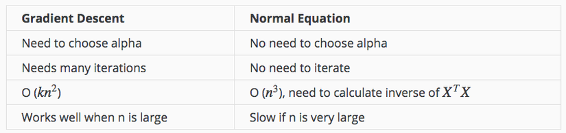
With the normal equation, computing the inversion has complexity O(n3). So if we have a very large number of features, the normal equation will be slow. In practice, when n exceeds 10,000 it might be a good time to go from a normal solution to an iterative process.

If XTX is noninvertible, the common causes might be having :

Redundant features, where two features are very closely related (i.e. they are linearly dependent) Too many features (e.g. m ≤ n). In this case, delete some features or use "regularization" . Solutions to the above problems include deleting a feature that is linearly dependent with another or deleting one or more features when there are too many features.