Thiết kế mạng Quantum Neural Network với Pytorch và Qiskit

ContentCreator

Mở đầu

Ở các phần trước, mình đã giới thiệu qua về lý thyết cơ bản để xây dựng một mạng nơ-ron lượng tử đồng thời kết hợp code ví dụ với thư viện Paddle Quantum. Tiếp tục với chuỗi bài về mạng nơ-ron lượng tử, ở phần này mình sẽ giới thiệu tới các bạn cách xây dựng QNN với một thư viện khá quen thuộc trong lĩnh vực Deep Learning đó là Pytorch, kết hợp với framework Qiskit được cung cấp bởi IBM. Tuy nhiên vẫn phải lưu ý là toàn bộ phần code này có thể chạy trên colab notebook chứ không phải máy tính lượng tử nên các bạn có thể yên tâm chạy thử nhé !

Cách thức hoạt động

Về cơ bản thì mô hình QNN (Quantum Neural Network) về cơ bản vẫn sẽ có 2 phần : phần chính là classical layer và phần phụ là quantum layer. Nói đến đây thì một số bạn có thể thắc mắc là tại sao mạng nơ-ron lượng tử mà thành phần chính lại không phải các quantum layer? Chúng ta hoàn toàn có thể xây dựng một mạng nơ-ron thuần quantum, nhưng khối lượng tính toán sẽ cực kỳ lớn khiến thời gian training với máy tính thường khá lâu, không thích hợp cho nội dung mình muốn truyền tải nên tạm thời mình sẽ để quantum layer đóng vai ít quan trọng đồng thời cũng sẽ có so sánh với mạng nơ-ron thông thường để các bạn thấy lợi ích và "tác hại" của lượng tử nhé :v

Để thiết kế mạng QNN thì với những ai đã quen thuộc với thư viện Pytorch, chúng ta có thể đơn giản tưởng tượng cách thiết kế y hệt một mạng NN thông thường, chỉ khác ở chỗ ta sẽ thêm một quantum layer vào một vị trí nào đấy trong mạng. Quantum layer mà mình sử dụng ở đây là một mạch tham số hóa lượng tử (Parameterized Quantum Circuit - PQC). Mạch này nhận đầu ra từ một classical layer trong mạng, tính toán trong trường không gian $Hilbert$ và sau đó measure ra các giá trị thông thường.

Vậy quá trình backprop sẽ diễn ra như thế nào với quantum layer ? Mục đích của bài viết đơn giản là tạo một mạng QNN, nghiêng về phần code nhiều hơn là học thuật nên mình sẽ không nói quá dài về backpropagation cho quantum layer nhé. Dựa theo công trình nghiên cứu Parameter Shift Rule thì chúng ta có thể đúc kết ra công thức tính gradient cho quantum layer tại điểm $\theta$ như sau :

$\nabla_{\theta} \ \text{Quantum Circuit} = \text{Quantum Circuit} (\theta + s) - \text{Quantum Circuit} (\theta - s)$

Thực hành

Bước 1 : trước tiên chúng ta cần một số cài đặt một số thư viện cần dùng với cú pháp :

%pip install qiskit==0.30.0 pylatexenc

Bước 2 : Sau đó import các thư viện cần thiết:

import numpy as np
import matplotlib.pyplot as plt

import torch
from torch.autograd import Function
import torch.optim as optim
import torch.nn as nn
import torch.nn.functional as F
from torch.autograd import Variable

import qiskit
from qiskit import transpile, assemble

from qiskit.visualization import plot_state_qsphere,plot_histogram, plot_bloch_multivector, plot_state_city

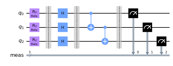
Bước 3 : một trong những bước quan trọng nhất - tạo Quantum Circuit. Circuit mà mình tạo khá đơn giản, đầu tiên sẽ nhận đầu vào thông qua cổng $R_Y$ nhằm biến đổi giá trị thực sang một trạng thái lượng tử, phương pháp xử lý dữ liệu này được gọi là "Angle Encoding". Với phương pháp này, chúng ta có thể tùy ý sử dụng một trong 3 cổng xoay $R_X, R_Y, R_Z$ . Tiếp theo đó, mình sử dụng 2 cổng $H$ và $CNOT$ để tạo rối lượng tử và cuối cùng là phép measure với cơ sở $Z$ : $\sigma_\mathbf{z} = \sum_i z_i p(z_i)$ . Như vậy là mình đã tạo một Quantum Circuit đơn giản đóng vai trò quantum layer trong mạng, lưu ý là ở đây mình có sử dụng cổng 2 qubit $CNOT$ vì thế nên mạch sẽ chỉ hoạt động với 2 qubit trở lên, chính xác hơn thì trong bài này mình sẽ sử dụng 3 qubit để xây dựng mạch.

Mạch trên được tạo như sau:

circuit = qiskit.QuantumCircuit(n_qubits)
n_qubits = n_qubits
theta = qiskit.circuit.Parameter('theta')
        
all_qubits = [i for i in range(n_qubits)]
circuit.ry(self.theta, all_qubits)
circuit.barrier()
circuit.h(all_qubits)
circuit.barrier()
for k in range(n_qubits-1):
       self.circuit.cx(k, k+1)
circuit.measure_all()

Kết quả:

Đưa đoạn code này vào class để tiện sử dụng :

class SimpleCircuit:
    """ 
    This class provides a simple interface for interaction 
    with the quantum circuit 
    """
    
    def __init__(self, n_qubits, backend, shots, n_input=9):
        # --- Circuit definition ---

        self.n_qubits=n_qubits
        self.n_inputs = n_input

        self.circuit = qiskit.QuantumCircuit(n_qubits)
        self.n_qubits = n_qubits
        self.theta = qiskit.circuit.Parameter('theta')
        
        all_qubits = [i for i in range(n_qubits)]
        self.circuit.ry(self.theta, all_qubits)
        self.circuit.barrier()
        self.circuit.h(all_qubits)
        self.circuit.barrier()
        for k in range(n_qubits-1):
            self.circuit.cx(k, k+1)

        self.circuit.measure_all()

        # ---------------------------

        self.backend = backend
        self.shots = shots
    
    def forward(self, thetas):
        t_qc = transpile(self.circuit,
                         self.backend)
        qobj = assemble(t_qc,
                        shots=self.shots,
                        parameter_binds = [{self.theta: theta.item()} for theta in thetas])
        job = self.backend.run(qobj)
        result = job.result().get_counts()
        exp = []
        for dict_ in result:
            counts = np.array(list(dict_.values()))
            states = np.array([int(k,2) for k in list(dict_.keys())])
            probabilities = counts / self.shots
            expectation = states * probabilities
            while expectation.shape[0]<2**self.n_qubits:
                expectation = np.append(expectation, 0.00)
            exp.append(expectation)
   
        return np.asarray(exp).T.sum(0)
    def plot(self, thetas):
        self.plot_backend = qiskit.Aer.get_backend("statevector_simulator")
        t_qc = transpile(self.circuit,
                         self.plot_backend)
        qobj = assemble(t_qc,
                        shots=self.shots,
                        parameter_binds = [{self.theta: theta.item()} for theta in thetas])
        job = self.plot_backend.run(qobj)
        result = job.result().get_counts()[0]

        display(plot_state_qsphere(job.result().get_statevector(0)))
        display(plot_state_city(job.result().get_statevector(0), figsize=[16, 9]))
        display(self.circuit.draw("mpl"))
        display(plot_histogram(job.result().get_counts()[0]))

Ở đoạn code trên thì nội dung trong hàm init mình đã giới thiệu trước rồi nên bỏ qua nhé. Hàm forward nhận đầu vào là tensor có số chiều $(1,N)$ . Sau đó lần lượt forward tensor này qua 3 cổng $R_Y$ ở 3 qubit : parameter_binds = [{self.theta: theta.item()} for theta in thetas]). Từ đó mạch sẽ tiến hành tính toán và measure đầu ra result dưới dạng các dictionary với key là chuỗi bit '000' -> '111' và result là xác suất rơi vào 1 trong 8 trạng thái trên, sau đó ta sẽ lợi dụng những giá trị này để tạo đầu ra mong muốn

Bước 4 : Sau khi tạo quantum circuit, chúng ta có thể tiến đến bước "bọc" circuit với thư viện Pytorch cho quá trình forward và backward tương tự như một dense layer bình thường:

class TorchCircuit(Function):    

    @staticmethod
    def forward(ctx, inp, circuit=None, shift=np.pi/2):
        if not hasattr(ctx, 'QiskitCirc'):
            ctx.QiskitCirc = SimpleCircuit(NUM_QUBITS, SIMULATOR, shots=NUM_SHOTS, n_input=NUM_INP)
            
        exp_value = ctx.QiskitCirc.forward(inp)
        
        result = torch.tensor([exp_value])
        
        
        ctx.save_for_backward(result, inp)
        
        return result
    
    @staticmethod
    
    def backward(ctx, grad_output):
        
        forward_tensor, i = ctx.saved_tensors
        input_numbers = i
        gradients = torch.Tensor()
        
        for k in range(NUM_INP):
            shift_right = input_numbers.detach().clone()
            shift_right[k] = shift_right[k] + SHIFT
            shift_left = input_numbers.detach().clone()
            shift_left[k] = shift_left[k] - SHIFT
            
            
            expectation_right = ctx.QiskitCirc.forward(shift_right)
            expectation_left  = ctx.QiskitCirc.forward(shift_left)
            gradient = torch.tensor([expectation_right]) - torch.tensor([expectation_left])
            gradients = torch.cat((gradients, gradient.float()))
        result = torch.Tensor(gradients)

        return (result.float() * grad_output.float()).T

Đồng thời define một số hyperparameter:

NUM_INP=10           
NUM_QUBITS = 3
SIMULATOR=qiskit.Aer.get_backend('qasm_simulator')

NUM_SHOTS=512
SHIFT = np.pi/2
n_samples = 150

Bước 5 : chuẩn bị dữ liệu. Bộ dữ liệu mà mình sử dụng là tập mnist 60000 sample được thu thập từ khoảng 250 người viết., tuy nhiên mình chỉ sử dụng 1500 sample train và 1500 sample test mỗi class. Vì thời gian training khá lâu nên mình sẽ sử dụng hạn chế nhất lượng dữ liệu cần dùng để tăng tốc quá trình training.

import numpy as np
import torchvision
from torchvision import datasets, transforms


X_train = datasets.MNIST(root='./data', train=True, download=True,
                         transform=transforms.Compose([transforms.ToTensor()]))

idx = np.append(np.where(X_train.targets == 0)[0][:n_samples], 
                np.where(X_train.targets == 1)[0][:n_samples])
idx = np.append(idx, 
                np.where(X_train.targets == 2)[0][:n_samples])
idx = np.append(idx, 
                np.where(X_train.targets == 3)[0][:n_samples])
idx = np.append(idx, 
                np.where(X_train.targets == 4)[0][:n_samples])
idx = np.append(idx, 
                np.where(X_train.targets == 5)[0][:n_samples])
idx = np.append(idx, 
                np.where(X_train.targets == 6)[0][:n_samples])
idx = np.append(idx, 
                np.where(X_train.targets == 7)[0][:n_samples])
idx = np.append(idx, 
                np.where(X_train.targets == 8)[0][:n_samples])
idx = np.append(idx, 
                np.where(X_train.targets == 9)[0][:n_samples])

X_train.data = X_train.data[idx]
X_train.targets = X_train.targets[idx]


train_loader = torch.utils.data.DataLoader(X_train, batch_size=1, shuffle=True, pin_memory=True)


X_test = datasets.MNIST(root='./data', train=False, download=True,
                        transform=transforms.Compose([transforms.ToTensor()]))

idx = np.append(np.where(X_test.targets == 0)[0][:n_samples], 
                np.where(X_test.targets == 1)[0][:n_samples])
idx = np.append(idx, 
                np.where(X_test.targets == 2)[0][:n_samples])
idx = np.append(idx, 
                np.where(X_test.targets == 3)[0][:n_samples])
idx = np.append(idx, 
                np.where(X_test.targets == 4)[0][:n_samples])
idx = np.append(idx, 
                np.where(X_test.targets == 5)[0][:n_samples])
idx = np.append(idx, 
                np.where(X_test.targets == 6)[0][:n_samples])
idx = np.append(idx, 
                np.where(X_test.targets == 7)[0][:n_samples])
idx = np.append(idx, 
                np.where(X_test.targets == 8)[0][:n_samples])
idx = np.append(idx, 
                np.where(X_test.targets == 9)[0][:n_samples])

X_test.data = X_test.data[idx]
X_test.targets = X_test.targets[idx]

test_loader = torch.utils.data.DataLoader(X_test, batch_size=1, shuffle=True)

Bước 6 : Dựng model với quantum layer đóng vai trò là layer cuối có nhiệm vụ prediction

class Net(nn.Module):
    def __init__(self):
        super(Net, self).__init__()
        self.conv1 = nn.Conv2d(1, 10, kernel_size=5)
        self.conv2 = nn.Conv2d(10, 20, kernel_size=5)
        self.conv2_drop = nn.Dropout2d()
        self.fc1 = nn.Linear(320, 50)
        self.fc2 = nn.Linear(50, NUM_INP)
        self.qc = TorchCircuit.apply
        self.qcsim = nn.Linear(NUM_INP, NUM_INP)
        self.fc3 = nn.Linear(NUM_INP, 10)

    def forward(self, x):
        x = F.relu(F.max_pool2d(self.conv1(x), 2))
        x = F.relu(F.max_pool2d(self.conv2_drop(self.conv2(x)), 2))
        x = x.view(-1, 320)
        x = F.relu(self.fc1(x))
        x = F.dropout(x, training=self.training)
        x = self.fc2(x)
        x = np.pi*torch.tanh(x)
        
#         print('params to QC: {}'.format(x))

        MODE = 'QC' # 'QC' or 'QC_sim'
    
        if MODE == 'QC': 
            x = torch.cat([self.qc(x_i) for x_i in x]) # QUANTUM LAYER
            print(self.qc(x[0]).shape)
        else:
            x = self.qcsim(x)


        # x = F.relu(self.fc3(x.float()))
        # x = torch.cat((x, 1-x), -1)
        return x

    def predict(self, x):
        # apply softmax
        pred = self.forward(x)
#         print(pred)
        ans = torch.argmax(pred[0]).item()
        return torch.tensor(ans)

Bước 7 : thiết kế training script và bắt đầu quá trình training

from tqdm import tqdm
epochs = 10
loss_list = []
loss_func = nn.CrossEntropyLoss()
list_acc = []

for epoch in range(epochs):
    total_loss = []
    for batch_idx, (data, target) in enumerate(tqdm(train_loader)):
#         print(batch_idx)
        optimizer.zero_grad()        
        # Forward pass
        output = network(data)
        # Calculating loss
        loss = loss_func(output, target)
        # Backward pass
        loss.backward()
        # Optimize the weights
        optimizer.step()
        total_loss.append(loss.item())
        
    loss_list.append(sum(total_loss)/len(total_loss))
    print('Training [{:.0f}%]\tLoss: {:.4f}'.format(
        100. * (epoch + 1) / epochs, loss_list[-1]))
    torch.save({
            'epoch': epoch,
            'model': network.state_dict(),
            'optimizer_state_dict': optimizer.state_dict(),
            'loss': loss.item(),
            }, f"/content/gdrive/MyDrive/Adhoc/model_quantum_{epoch}.pth")
    accuracy = 0
    number = 0
    network.eval()
    for batch_idx, (data, target) in enumerate(test_loader):
        number +=1
        output = network(data)
        accuracy += (output.argmax(1) == target[0].item())
        # accuracy += (output.argmax(1).cpu() == target.cpu()).sum().item()
    print("Performance on test data is : {}/{} = {}%".format(accuracy,number,100*accuracy/number))
    list_acc.append(100*accuracy.item()/number)

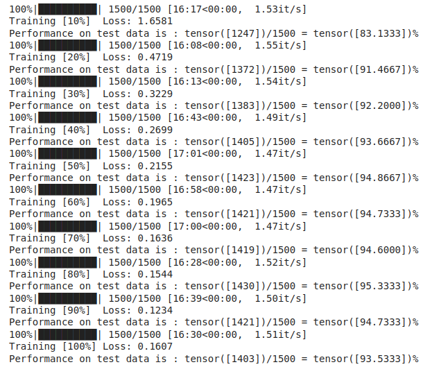
Và đây là thành quả cuối cùng:

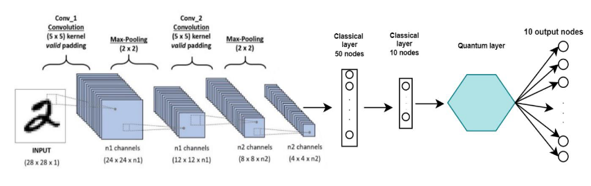
Toàn bộ model của mình có thể được mô hình hóa lại như sau:

So sánh thời gian training giữa mô hình thông thường và mô hình lượng tử thì mô hình CNN thông thường chỉ mất 1 phút cho 10 epoch với lượng dữ liệu trên, trong khi mô hình lượng tử mất gần 2 tiếng :V Nhưng kết quả mang lại thì khá tương xứng với công sức bỏ ra khi accuracy của QNN hoàn toàn vượt trội so với CNN thông thường. Tuy đạt được mục tiêu đề ra, nhưng do hạn chế về mặt thời gian thực hiện, bài viết vẫn chưa phát triển được hết các tính năng của Quantum Neural Network, cụ thể là mới triển khai được trên máy tính thông thường, còn việc huấn luyện và kiểm thử mô hình trên máy lượng tử thì vẫn chưa được triển khai. Trong tương lai, nếu có cơ hội, mình sẽ tiếp tục nghiên cứu và phát triển các loại Quantum Neural Network với nhiều bài toán phức tạp hơn.