Support Vector Machines
Bài đăng này đã không được cập nhật trong 4 năm
Introduction to Support Vector Machine(SVM)
A Support Vector Machine (SVM) is a supervised machine learning algorithm that can be employed for both classification and regression purposes. However, it is mostly used in classification problems. In this algorithm, we plot each data item as a point in n-dimensional space (where n is number of features you have) with the value of each feature being the value of a particular coordinate. Then, we perform classification by finding the hyper-plane that differentiate the two classes very well. Support Vectors are simply the co-ordinates of individual observation.
Optimization Objective
In order to describe the support vector machine, I'm actually going to start with logistic regression, and show how we can modify it a bit, and get what is essentially the support vector machine. For details to logistic regression model please refer to ......
Our hypothesis for logistic regression is
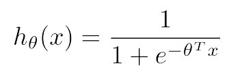 and sigmoid activation function
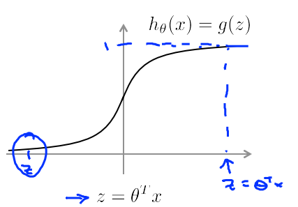 here z is used to denote theta transpose axiom.
From the graph we can see that, If we have an example with y equals one we're sort of hoping that h of x will be close to one.So,theta transpose x or z must be much larger than 0.The greater the value of theta transpose of x the farther the z goes to right.Therefore, the outputs of logistic progression becomes close to one.
here z is used to denote theta transpose axiom.
From the graph we can see that, If we have an example with y equals one we're sort of hoping that h of x will be close to one.So,theta transpose x or z must be much larger than 0.The greater the value of theta transpose of x the farther the z goes to right.Therefore, the outputs of logistic progression becomes close to one.
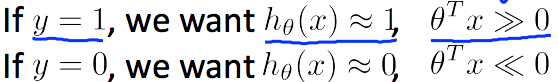 Conversely, if we have an example where y is equal to zero, then what we're hoping for is that the hypothesis will output a value close to zero. And that corresponds to theta transpose x of z being much less than zero because that corresponds to a hypothesis of putting a value close to zero.
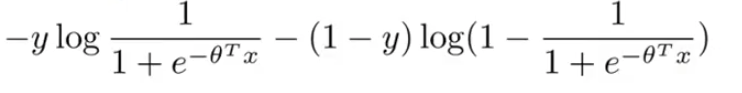
Now if we consider cost function of logistic regression for a single training sample we have,
Conversely, if we have an example where y is equal to zero, then what we're hoping for is that the hypothesis will output a value close to zero. And that corresponds to theta transpose x of z being much less than zero because that corresponds to a hypothesis of putting a value close to zero.
Now if we consider cost function of logistic regression for a single training sample we have,
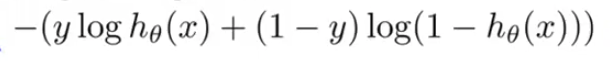 If we plug our hypothesis function to the cost function we get,
 For y =1, only the first term in the objective matters, because one minus y term would be equal to zero if y is equal to one.
For y = 0, the the 2nd term matters as first term gets eliminated.
For y =1, only the first term in the objective matters, because one minus y term would be equal to zero if y is equal to one.
For y = 0, the the 2nd term matters as first term gets eliminated.
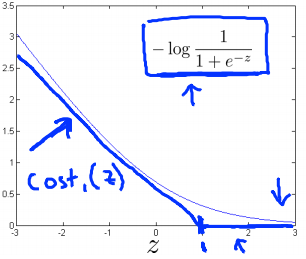
in case of y =1, if theta transpose x or z is very large it corresponds to very small value of cost function. Now for support vector machine we take a bit modified graph.
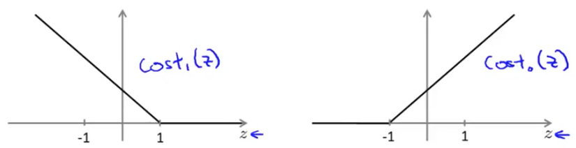
We make use of two flat line to represent the same curve like in the graph. This will give us computaional advantage and easier optimization.
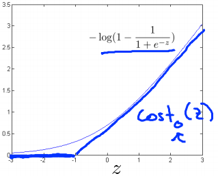 in case of y =0, if theta transpose x or z is very small it corresponds to very small value of cost function.We draw two flat lines almost in the same way like before. Now we name the first and second line graph as cost1 of z for y=1 and cost0 of z for y=0.
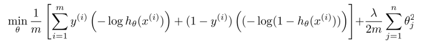
Now in logistic regression we have cost function like for minimizing cost over m training data, where first part is from training set and second part is regularization parameter part
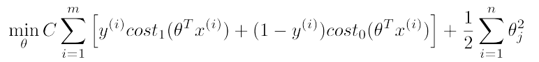
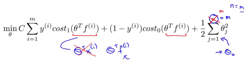
 In Support Vector Machine we just replace the hypothesis suntion with our new cost1 and cost0 functions with slightly differently re-parameterized.First, we can get rid of the 1/m term as there is no point of multiplying constant which you are already minimizing over.To trade of relative weight between first term and 2nd term of the function we're instead going to use a different parameter which by convention is called C and is set to minimize CA + B instead of A + lambda.B . So in SVM, instead of using lambda here to control the relative waiting between the first and second terms.So this is just a different way of controlling the trade off, it's just a different way of prioritizing how much we care about optimizing the first term, versus how much we care about optimizing the second term. And if you want you can think of this as the parameter C playing a role similar to 1 over lambda. So instead of lamba we are going to use C here and get our new cost function for SVM.
SVM as Large Margin Classifier
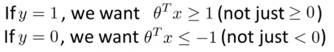 if y is equal to 1, then cost1 of Z is zero only when Z is greater than or equal to 1. So in other words, if you have a positive example, we really want theta transpose x to be greater than or equal to 1 and conversely if y is equal to zero.
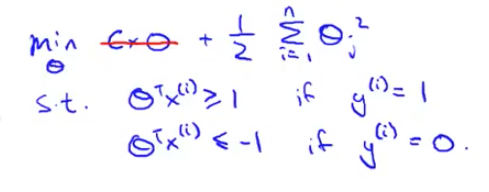
Let's consider a case ,where we set constant C to be a very large value, so let's imagine we set C to a very large value, may be a hundred thousand, some huge number. If C is very, very large, then when minimizing this optimization objective, we're going to be highly motivated to choose a value, so that this first term is equal to zero. So let's try to understand the optimization problem in the context of, what would it take to make this first term in the objective equal to zero.We saw already that whenever we have a training example with a label of y=1 if we want to make that first term zero, what we need is is to find a value of theta so that theta transpose x i is greater than or equal to 1. And similarly, whenever we have an example, with label zero, in order to make sure that the cost, cost0 of Z, in order to make sure that cost is zero we need that theta transpose x is less than or
equal to -1. So, if we think of our optimization problem as now, really choosing parameters and show that this first term is equal to zero, what we're left with is the optimization problem.
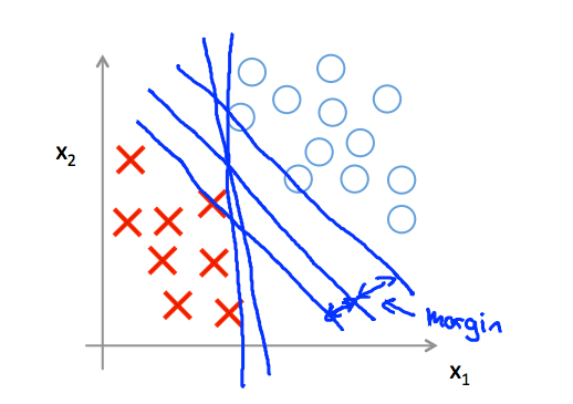
For data set , like positive and negative samples below which are linearly separable, SVM will choose the line whice separates the data in a way that it maintains a minimum distance or margin from the line.For maintaining this margin, SVM is sometimes called large margin classfier. This margin this gives the SVM a certain robustness, because it tries to separate the data with as a large a margin as possible.
Kernels
For adapting support vector machines in order to develop complex nonlinear classifiers there is a technique called kernels.
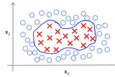
If we have a training set that looks like this, and we want to find a nonlinear decision boundary to distinguish the positive and negative examples. One way to do so is to come up with a set of complex polynomial features. For example -
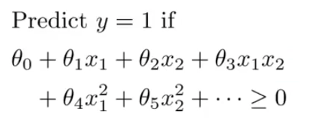
And another way of writing this, to introduce a level of new notation is substituting features with f1,f2,f3,..... so that x1 = f1, x2 = f2, f1 = x1x2, ... and so on. So higher order polynomials is one way to come up with more features.But using high order polynomials becomes very computationally expensive because there are a lot of these higher order polynomial terms. So we have to think of better ways to choosing features.
For now, ignoring x0 and considering only x1, x2, x3 features and manually pick a few points, and then call these points l1, l2, l3.
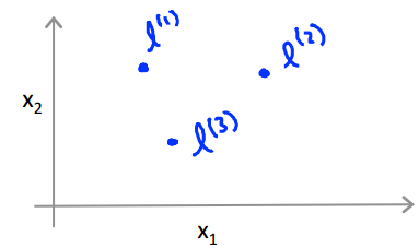
and define new features as follows, given an example X, define first feature f1 to be some measure of the similarity between training example X and first landmar l1 k and this specific formula that measure similarity is going to be like below and so are features f2 and f3
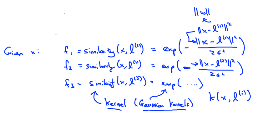
in this case the similarity function is actually Gaussian kernel and squared ||x-l1|| is actualy euclidian distance.
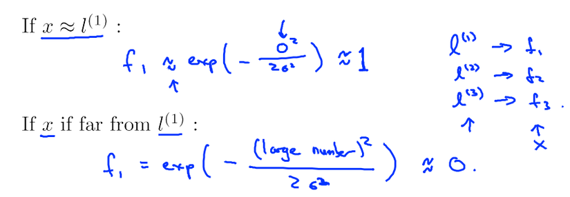
Now for example, if X is near l1 then f1 will be approximately 1 and if its far from l1 then f1 will beapproximately 0
 For choosing the landmarks we are going to put the landmarks in the same locations of the training examples, so we are going to have l1,l2,....lm landmarks for m training examples.So if we have one training example if that is x1, well then we are going to choose this first landmark to be at xactly the same location as our first training example.
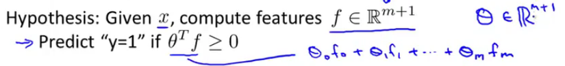
and we are gong to have a feature vector of f0, f1, f2,....fm.
For choosing the landmarks we are going to put the landmarks in the same locations of the training examples, so we are going to have l1,l2,....lm landmarks for m training examples.So if we have one training example if that is x1, well then we are going to choose this first landmark to be at xactly the same location as our first training example.
and we are gong to have a feature vector of f0, f1, f2,....fm.
So now the hypothesis becomes
 and cost function becomes like,
When using an SVM, one of the things we need to choose is the parameter C which was in the optimization objective, and we recall that C played a role similar to 1 over lambda, where lambda was the regularization parameter we had for logistic regression. So, if we have a large value of C, this corresponds to what we have back in logistic regression, of a small value of lambda meaning of not using much regularization. And if we do that, we tend to have a hypothesis with lower bias and higher variance.
if we use a smaller value of C then this corresponds to when we are using logistic regression with a large value of lambda and that corresponds to a hypothesis with higher bias and lower variance. And so, hypothesis with large C has a higher variance, and is more prone to overfitting, whereas hypothesis with small C has higher bias and is thus more prone to underfitting.
The other one is the parameter sigma squared, which appeared in the Gaussian kernel. if sigma squared is large, then, you know, the Gaussian kernel would tend to fall off relatively slowly and falls sharply if small.
All rights reserved
