Paper reading | GRAPH ATTENTION NETWORKS
Bài đăng này đã không được cập nhật trong 2 năm
Giới thiệu
Các mô hình CNN thể hiện sự mạnh mẽ khi áp dụng vào những bài toán có dữ liệu là hình ảnh ví dụ như image classification, semantic segmentation, object detection,... trong đó dữ liệu hình ảnh có biểu diễn cấu trúc ở dạng lưới. Khi đó, ta có thể sử dụng các filter (bộ lọc) trong mạng CNN trượt qua hình ảnh để trích xuất các đặc trưng. Tuy nhiên, dữ liệu có những biểu diễn phức tạp hơn trong thực tế ví dụ như ở dạng đồ thị (graph) cụ thể là dữ liệu về mạng xã hội, mạng viễn thông, dữ liệu y sinh như cấu trúc ADN,...
Để xử lý dữ liệu graph nhiều kiến trúc mạng neural network ra đời. Sớm nhất ta có Recursive Neural Network được sử dụng để xử lý dữ liệu được biểu diễn trong một đồ thị tuần hoàn có hướng (Directed Acyclic Graph - DAG). Sau đó là Graph Neural Networks (GNNs) có thể xử lý nhiều loại graph hơn như đồ thị vô hướng, đồ thị có hướng, đồ thị tuần hoàn. Bên cạnh đó, các nghiên cứu về việc tổng quát hoá tích chập (convolution) để sử dụng cho dữ liệu graph cũng được quan tâm. Tuy nhiên trong Graph Convolutional Networks (GCN), các node hàng xóm lại được biểu diễn với mức độ quan trọng là như nhau. Việc sử dụng GCN sẽ làm giảm độ chính xác trong các bài toán có dữ liệu mà trong đó các node có mức độ ảnh hưởng khác nhau tới các node còn lại.
Đóng góp của bài báo
Bài báo đề xuất Graph Attention Networks (GAT) giúp giải quyết vấn đề của GCN. Để xét tới mức độ quan trọng của các node hàng xóm, cơ chế attention được sử dụng để chỉ định trọng số của từng kết nối (connection) giữa các node. Ý tưởng chính là mô hình thực hiện tính toán biểu diễn của từng node dựa vào các node hàng xóm theo một chiến lược self-attention. Việc sử dụng chiến lược self-attention cho graph có một số đặc điểm hay ho sau:
- Việc tính toán có thể thực hiện song song trên các cặp node láng giềng
- Có thể áp dụng cho các node có số node hàng xóm khác nhau (hay degree khác nhau) bằng cách đánh trọng số cho các node hàng xóm
- Mô hình có thể áp dụng trực tiếp vào các bài toán inductive learning, bao gồm các nhiệm vụ trong đó mô hình phải tổng quát hóa cho các đồ thị hoàn toàn không được nhìn thấy trước đó
Kiến trúc GAT
Graph attentional layer
Trước khi đi vào GAT layer, ta sẽ cùng tìm hiểu lại cơ chế hoạt động của GCN layer. GCN layer được biểu diễn bằng một công thức toán học như sau:
trong đó:
- là node feature của node thứ tại layer
- là tập các node hàng xóm của node . Trong tập này bao gồm cả chính node mà ta đang xét
- là hằng số chuẩn hóa dựa trên cấu trúc đồ thị, định nghĩa phép tính trung bình đẳng hướng.
- là hàm activation thực hiện biến đổi phi tuyến tính
- là ma trận trọng số learnable sử dụng cho feature transformation
Đầu vào của graph attentional layer là một tập các node feature trong đó là số node và là số lượng feature trong mỗi node. Mục tiêu của graph attentional layer (GAT layer) là tạo ra một tập các node feature mới .
Đầu tiên, ta sử dụng một lớp biến đổi tuyến tính để biến đổi từ feature đầu vào sang high-level feature. Sau đó ta sử dụng cơ chế attention trên các high-level feature để tính attention coefficient (hệ số chú ý) giữa các cặp node dựa vào feature của chúng.
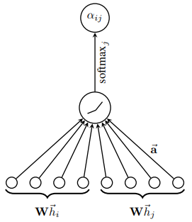
Các coefficient này sau đó thường được chuẩn hóa bằng hàm softmax để có thể so sánh dễ dàng giữa các node hàng xóm khác nhau:
Về bản chất, cơ chế attention chỉ là một layer được tham số hóa bởi vector trọng số , sau đó sử dụng hàm activation LeakyReLU. Tất cả được thể hiện trong công thức dưới đây 
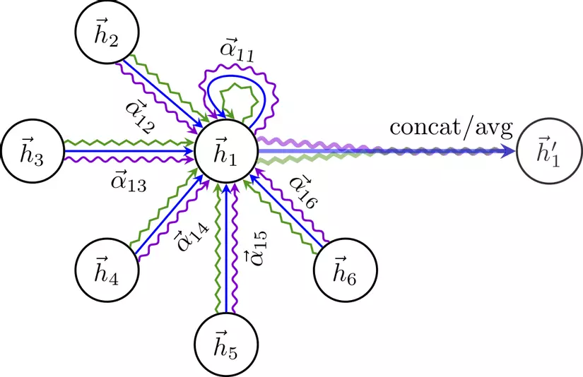
Để quá trình học của self-attention được ổn định, nhóm tác giả nhận thấy rằng việc sử dụng multi-head attention mang lại nhiều lợi ích. Cụ thể, các operation của cơ chế attention được sao chép độc lập lần. Mỗi bản sao sẽ có các bộ weight riêng, nghĩa là chúng học cách tạo ra các output độc lập. Đầu ra cuối cùng sẽ được tổng hợp thông qua một phép cộng hoặc concat.
Nếu như ta thực hiện multi-head attention trên layer cuối của mạng, việc sử dụng concat sẽ không còn hợp lý. Thay vào đó, ta sử dụng phép tính trung bình cộng và sau đó mới dùng một hàm phi tuyến tính (ví dụ như softmax hoặc sigmoid nếu cho bài toán phân loại). Công thức như sau:
Hình dưới mô tả toàn bộ quá trình trên. Ở đây ta thực hiện sử dụng multi-head attention (với số head là ) trên node 1 với các node hàng xóm của nó. Feature của mỗi head được concat hoặc tính trung bình để cho ra feature cuối cùng.
Tóm tắt đặc điểm của layer GAT
Một số đặc điểm của layer GAT:
- Hiệu suất tính toán: Quá trình tính toán các hệ số attention ý có thể được tính toán song song trên tất cả các cạnh của đồ thị và quá trình tổng hợp cũng có thể được thực hiện song song trên tất cả các node. Độ phức tạp của một GAT head có đầu ra là feature là , trong đó là số lượng input feature. và là số lượng node và cạnh trong graph. Độ phức tạp này tương đương với GCN. Khi áp dụng multi-head attention sẽ làm tăng bộ nhớ và tham số lên lần ( là số head), tuy nhiên tốc độ tính toán lại tương đương như khi sử dụng 1 head do có thể thực hiện tính toán song song.
- Số lượng tham số cố định, không phụ thuộc vào số node hoặc số cạnh của đồ thị
- Dễ dàng cục bộ hóa, vì ta chỉ chú ý đến node hàng xóm
- Cho phép xác định mức độ quan trọng khác nhau cho các node hàng xóm khác nhau
- Dễ áp dụng cho các inductive problem, vì nó là một cơ chế chia sẻ trên cạnh và do đó không phụ thuộc vào cấu trúc đồ thị toàn cục
Coding
import torch
import torch.nn as nn

from utils.constants import LayerType

class GAT(torch.nn.Module):
    """
    3 GAT implementations
    """

    def __init__(self, num_of_layers, num_heads_per_layer, num_features_per_layer, add_skip_connection=True, bias=True,
                 dropout=0.6, layer_type=LayerType.IMP3, log_attention_weights=False):
        super().__init__()
        assert num_of_layers == len(num_heads_per_layer) == len(num_features_per_layer) - 1, f'Enter valid arch params.'

        GATLayer = get_layer_type(layer_type)  # fetch one of 3 available implementations
        num_heads_per_layer = [1] + num_heads_per_layer  # trick - so that we can nicely create GAT layers below

        gat_layers = []  # collect GAT layers
        for i in range(num_of_layers):
            layer = GATLayer(
                num_in_features=num_features_per_layer[i] * num_heads_per_layer[i],  # consequence of concatenation
                num_out_features=num_features_per_layer[i+1],
                num_of_heads=num_heads_per_layer[i+1],
                concat=True if i < num_of_layers - 1 else False,  # last GAT layer does mean avg, the others do concat
                activation=nn.ELU() if i < num_of_layers - 1 else None,  # last layer just outputs raw scores
                dropout_prob=dropout,
                add_skip_connection=add_skip_connection,
                bias=bias,
                log_attention_weights=log_attention_weights
            )
            gat_layers.append(layer)

        self.gat_net = nn.Sequential(
            *gat_layers,
        )

    def forward(self, data):
        return self.gat_net(data)


class GATLayer(torch.nn.Module):
    """
    Base class for all implementations as there is much code that would otherwise be copy/pasted.
    """

    head_dim = 1

    def __init__(self, num_in_features, num_out_features, num_of_heads, layer_type, concat=True, activation=nn.ELU(),
                 dropout_prob=0.6, add_skip_connection=True, bias=True, log_attention_weights=False):

        super().__init__()

        self.num_of_heads = num_of_heads
        self.num_out_features = num_out_features
        self.concat = concat  # whether we should concatenate or average the attention heads
        self.add_skip_connection = add_skip_connection

        #
        # Trainable weights: linear projection matrix (denoted as "W" in the paper), attention target/source
        # (denoted as "a" in the paper) and bias (not mentioned in the paper but present in the official GAT repo)
        #

        if layer_type == LayerType.IMP1:
            self.proj_param = nn.Parameter(torch.Tensor(num_of_heads, num_in_features, num_out_features))
        else:
            # You can treat this one matrix as num_of_heads independent W matrices
            self.linear_proj = nn.Linear(num_in_features, num_of_heads * num_out_features, bias=False)

        # After we concatenate target node (node i) and source node (node j) we apply the additive scoring function
        # which gives us unnormalized score "e". Here we split the "a" vector - but the semantics remain the same.

        # Basically instead of doing [x, y] (concatenation, x/y are node feature vectors) and dot product with "a"
        # we instead do a dot product between x and "a_left" and y and "a_right" and we sum them up
        self.scoring_fn_target = nn.Parameter(torch.Tensor(1, num_of_heads, num_out_features))
        self.scoring_fn_source = nn.Parameter(torch.Tensor(1, num_of_heads, num_out_features))

        if layer_type == LayerType.IMP1:  # simple reshape in the case of implementation 1
            self.scoring_fn_target = nn.Parameter(self.scoring_fn_target.reshape(num_of_heads, num_out_features, 1))
            self.scoring_fn_source = nn.Parameter(self.scoring_fn_source.reshape(num_of_heads, num_out_features, 1))

        # Bias is definitely not crucial to GAT - feel free to experiment
        if bias and concat:
            self.bias = nn.Parameter(torch.Tensor(num_of_heads * num_out_features))
        elif bias and not concat:
            self.bias = nn.Parameter(torch.Tensor(num_out_features))
        else:
            self.register_parameter('bias', None)

        if add_skip_connection:
            self.skip_proj = nn.Linear(num_in_features, num_of_heads * num_out_features, bias=False)
        else:
            self.register_parameter('skip_proj', None)

        #
        # End of trainable weights
        #

        self.leakyReLU = nn.LeakyReLU(0.2)  # using 0.2 as in the paper
        self.softmax = nn.Softmax(dim=-1)  # -1 stands for apply the log-softmax along the last dimension
        self.activation = activation
        self.dropout = nn.Dropout(p=dropout_prob)

        self.log_attention_weights = log_attention_weights  # whether we should log the attention weights
        self.attention_weights = None  # for later visualization purposes, I cache the weights here

        self.init_params(layer_type)

    def init_params(self, layer_type):
        nn.init.xavier_uniform_(self.proj_param if layer_type == LayerType.IMP1 else self.linear_proj.weight)
        nn.init.xavier_uniform_(self.scoring_fn_target)
        nn.init.xavier_uniform_(self.scoring_fn_source)

        if self.bias is not None:
            torch.nn.init.zeros_(self.bias)

    def skip_concat_bias(self, attention_coefficients, in_nodes_features, out_nodes_features):
        if self.log_attention_weights:  # potentially log for later visualization in playground.py
            self.attention_weights = attention_coefficients

        # if the tensor is not contiguously stored in memory we'll get an error after we try to do certain ops like view
        # only imp1 will enter this one
        if not out_nodes_features.is_contiguous():
            out_nodes_features = out_nodes_features.contiguous()

        if self.add_skip_connection:  # add skip or residual connection
            if out_nodes_features.shape[-1] == in_nodes_features.shape[-1]:  # if FIN == FOUT
                # unsqueeze does this: (N, FIN) -> (N, 1, FIN), out features are (N, NH, FOUT) so 1 gets broadcast to NH
                # thus we're basically copying input vectors NH times and adding to processed vectors
                out_nodes_features += in_nodes_features.unsqueeze(1)
            else:
                # FIN != FOUT so we need to project input feature vectors into dimension that can be added to output
                # feature vectors. skip_proj adds lots of additional capacity which may cause overfitting.
                out_nodes_features += self.skip_proj(in_nodes_features).view(-1, self.num_of_heads, self.num_out_features)

        if self.concat:
            # shape = (N, NH, FOUT) -> (N, NH*FOUT)
            out_nodes_features = out_nodes_features.view(-1, self.num_of_heads * self.num_out_features)
        else:
            # shape = (N, NH, FOUT) -> (N, FOUT)
            out_nodes_features = out_nodes_features.mean(dim=self.head_dim)

        if self.bias is not None:
            out_nodes_features += self.bias

        return out_nodes_features if self.activation is None else self.activation(out_nodes_features)


class GATLayerImp3(GATLayer):
    """
    Implementation #3 was inspired by PyTorch Geometric: https://github.com/rusty1s/pytorch_geometric

    It's suitable for both transductive and inductive settings. In the inductive setting we just merge the graphs
    into a single graph with multiple components and this layer is agnostic to that fact! <3
    """

    src_nodes_dim = 0  # position of source nodes in edge index
    trg_nodes_dim = 1  # position of target nodes in edge index

    nodes_dim = 0      # node dimension/axis
    head_dim = 1       # attention head dimension/axis

    def __init__(self, num_in_features, num_out_features, num_of_heads, concat=True, activation=nn.ELU(),
                 dropout_prob=0.6, add_skip_connection=True, bias=True, log_attention_weights=False):

        # Delegate initialization to the base class
        super().__init__(num_in_features, num_out_features, num_of_heads, LayerType.IMP3, concat, activation, dropout_prob,
                      add_skip_connection, bias, log_attention_weights)

    def forward(self, data):
        #
        # Step 1: Linear Projection + regularization
        #

        in_nodes_features, edge_index = data  # unpack data
        num_of_nodes = in_nodes_features.shape[self.nodes_dim]
        assert edge_index.shape[0] == 2, f'Expected edge index with shape=(2,E) got {edge_index.shape}'

        # shape = (N, FIN) where N - number of nodes in the graph, FIN - number of input features per node
        # We apply the dropout to all of the input node features (as mentioned in the paper)
        # Note: for Cora features are already super sparse so it's questionable how much this actually helps
        in_nodes_features = self.dropout(in_nodes_features)

        # shape = (N, FIN) * (FIN, NH*FOUT) -> (N, NH, FOUT) where NH - number of heads, FOUT - num of output features
        # We project the input node features into NH independent output features (one for each attention head)
        nodes_features_proj = self.linear_proj(in_nodes_features).view(-1, self.num_of_heads, self.num_out_features)

        nodes_features_proj = self.dropout(nodes_features_proj)  # in the official GAT imp they did dropout here as well

        #
        # Step 2: Edge attention calculation
        #

        # Apply the scoring function (* represents element-wise (a.k.a. Hadamard) product)
        # shape = (N, NH, FOUT) * (1, NH, FOUT) -> (N, NH, 1) -> (N, NH) because sum squeezes the last dimension
        # Optimization note: torch.sum() is as performant as .sum() in my experiments
        scores_source = (nodes_features_proj * self.scoring_fn_source).sum(dim=-1)
        scores_target = (nodes_features_proj * self.scoring_fn_target).sum(dim=-1)

        # We simply copy (lift) the scores for source/target nodes based on the edge index. Instead of preparing all
        # the possible combinations of scores we just prepare those that will actually be used and those are defined
        # by the edge index.
        # scores shape = (E, NH), nodes_features_proj_lifted shape = (E, NH, FOUT), E - number of edges in the graph
        scores_source_lifted, scores_target_lifted, nodes_features_proj_lifted = self.lift(scores_source, scores_target, nodes_features_proj, edge_index)
        scores_per_edge = self.leakyReLU(scores_source_lifted + scores_target_lifted)

        # shape = (E, NH, 1)
        attentions_per_edge = self.neighborhood_aware_softmax(scores_per_edge, edge_index[self.trg_nodes_dim], num_of_nodes)
        # Add stochasticity to neighborhood aggregation
        attentions_per_edge = self.dropout(attentions_per_edge)

        #
        # Step 3: Neighborhood aggregation
        #

        # Element-wise (aka Hadamard) product. Operator * does the same thing as torch.mul
        # shape = (E, NH, FOUT) * (E, NH, 1) -> (E, NH, FOUT), 1 gets broadcast into FOUT
        nodes_features_proj_lifted_weighted = nodes_features_proj_lifted * attentions_per_edge

        # This part sums up weighted and projected neighborhood feature vectors for every target node
        # shape = (N, NH, FOUT)
        out_nodes_features = self.aggregate_neighbors(nodes_features_proj_lifted_weighted, edge_index, in_nodes_features, num_of_nodes)

        #
        # Step 4: Residual/skip connections, concat and bias
        #

        out_nodes_features = self.skip_concat_bias(attentions_per_edge, in_nodes_features, out_nodes_features)
        return (out_nodes_features, edge_index)

    #
    # Helper functions (without comments there is very little code so don't be scared!)
    #

    def neighborhood_aware_softmax(self, scores_per_edge, trg_index, num_of_nodes):
        """
        As the fn name suggest it does softmax over the neighborhoods. Example: say we have 5 nodes in a graph.
        Two of them 1, 2 are connected to node 3. If we want to calculate the representation for node 3 we should take
        into account feature vectors of 1, 2 and 3 itself. Since we have scores for edges 1-3, 2-3 and 3-3
        in scores_per_edge variable, this function will calculate attention scores like this: 1-3/(1-3+2-3+3-3)
        (where 1-3 is overloaded notation it represents the edge 1-3 and it's (exp) score) and similarly for 2-3 and 3-3
         i.e. for this neighborhood we don't care about other edge scores that include nodes 4 and 5.

        Note:
        Subtracting the max value from logits doesn't change the end result but it improves the numerical stability
        and it's a fairly common "trick" used in pretty much every deep learning framework.
        Check out this link for more details:

        https://stats.stackexchange.com/questions/338285/how-does-the-subtraction-of-the-logit-maximum-improve-learning
        """

        # Calculate the numerator. Make logits <= 0 so that e^logit <= 1 (this will improve the numerical stability)
        scores_per_edge = scores_per_edge - scores_per_edge.max()
        exp_scores_per_edge = scores_per_edge.exp()  # softmax

        # Calculate the denominator. shape = (E, NH)
        neigborhood_aware_denominator = self.sum_edge_scores_neighborhood_aware(exp_scores_per_edge, trg_index, num_of_nodes)

        # 1e-16 is theoretically not needed but is only there for numerical stability (avoid div by 0) - due to the
        # possibility of the computer rounding a very small number all the way to 0.
        attentions_per_edge = exp_scores_per_edge / (neigborhood_aware_denominator + 1e-16)

        # shape = (E, NH) -> (E, NH, 1) so that we can do element-wise multiplication with projected node features
        return attentions_per_edge.unsqueeze(-1)

    def sum_edge_scores_neighborhood_aware(self, exp_scores_per_edge, trg_index, num_of_nodes):
        # The shape must be the same as in exp_scores_per_edge (required by scatter_add_) i.e. from E -> (E, NH)
        trg_index_broadcasted = self.explicit_broadcast(trg_index, exp_scores_per_edge)

        # shape = (N, NH), where N is the number of nodes and NH the number of attention heads
        size = list(exp_scores_per_edge.shape)  # convert to list otherwise assignment is not possible
        size[self.nodes_dim] = num_of_nodes
        neighborhood_sums = torch.zeros(size, dtype=exp_scores_per_edge.dtype, device=exp_scores_per_edge.device)

        # position i will contain a sum of exp scores of all the nodes that point to the node i (as dictated by the
        # target index)
        neighborhood_sums.scatter_add_(self.nodes_dim, trg_index_broadcasted, exp_scores_per_edge)

        # Expand again so that we can use it as a softmax denominator. e.g. node i's sum will be copied to
        # all the locations where the source nodes pointed to i (as dictated by the target index)
        # shape = (N, NH) -> (E, NH)
        return neighborhood_sums.index_select(self.nodes_dim, trg_index)

    def aggregate_neighbors(self, nodes_features_proj_lifted_weighted, edge_index, in_nodes_features, num_of_nodes):
        size = list(nodes_features_proj_lifted_weighted.shape)  # convert to list otherwise assignment is not possible
        size[self.nodes_dim] = num_of_nodes  # shape = (N, NH, FOUT)
        out_nodes_features = torch.zeros(size, dtype=in_nodes_features.dtype, device=in_nodes_features.device)

        # shape = (E) -> (E, NH, FOUT)
        trg_index_broadcasted = self.explicit_broadcast(edge_index[self.trg_nodes_dim], nodes_features_proj_lifted_weighted)
        # aggregation step - we accumulate projected, weighted node features for all the attention heads
        # shape = (E, NH, FOUT) -> (N, NH, FOUT)
        out_nodes_features.scatter_add_(self.nodes_dim, trg_index_broadcasted, nodes_features_proj_lifted_weighted)

        return out_nodes_features

    def lift(self, scores_source, scores_target, nodes_features_matrix_proj, edge_index):
        """
        Lifts i.e. duplicates certain vectors depending on the edge index.
        One of the tensor dims goes from N -> E (that's where the "lift" comes from).

        """
        src_nodes_index = edge_index[self.src_nodes_dim]
        trg_nodes_index = edge_index[self.trg_nodes_dim]

        # Using index_select is faster than "normal" indexing (scores_source[src_nodes_index]) in PyTorch!
        scores_source = scores_source.index_select(self.nodes_dim, src_nodes_index)
        scores_target = scores_target.index_select(self.nodes_dim, trg_nodes_index)
        nodes_features_matrix_proj_lifted = nodes_features_matrix_proj.index_select(self.nodes_dim, src_nodes_index)

        return scores_source, scores_target, nodes_features_matrix_proj_lifted

    def explicit_broadcast(self, this, other):
        # Append singleton dimensions until this.dim() == other.dim()
        for _ in range(this.dim(), other.dim()):
            this = this.unsqueeze(-1)

        # Explicitly expand so that shapes are the same
        return this.expand_as(other)


class GATLayerImp2(GATLayer):
    """
        Implementation #2 was inspired by the official GAT implementation: https://github.com/PetarV-/GAT

        It's conceptually simpler than implementation #3 but computationally much less efficient.

        Note: this is the naive implementation not the sparse one and it's only suitable for a transductive setting.
        It would be fairly easy to make it work in the inductive setting as well but the purpose of this layer
        is more educational since it's way less efficient than implementation 3.

    """

    def __init__(self, num_in_features, num_out_features, num_of_heads, concat=True, activation=nn.ELU(),
                 dropout_prob=0.6, add_skip_connection=True, bias=True, log_attention_weights=False):

        super().__init__(num_in_features, num_out_features, num_of_heads, LayerType.IMP2, concat, activation, dropout_prob,
                         add_skip_connection, bias, log_attention_weights)

    def forward(self, data):
        #
        # Step 1: Linear Projection + regularization (using linear layer instead of matmul as in imp1)
        #

        in_nodes_features, connectivity_mask = data  # unpack data
        num_of_nodes = in_nodes_features.shape[0]
        assert connectivity_mask.shape == (num_of_nodes, num_of_nodes), \
            f'Expected connectivity matrix with shape=({num_of_nodes},{num_of_nodes}), got shape={connectivity_mask.shape}.'

        # shape = (N, FIN) where N - number of nodes in the graph, FIN - number of input features per node
        # We apply the dropout to all of the input node features (as mentioned in the paper)
        in_nodes_features = self.dropout(in_nodes_features)

        # shape = (N, FIN) * (FIN, NH*FOUT) -> (N, NH, FOUT) where NH - number of heads, FOUT - num of output features
        # We project the input node features into NH independent output features (one for each attention head)
        nodes_features_proj = self.linear_proj(in_nodes_features).view(-1, self.num_of_heads, self.num_out_features)

        nodes_features_proj = self.dropout(nodes_features_proj)  # in the official GAT imp they did dropout here as well

        #
        # Step 2: Edge attention calculation (using sum instead of bmm + additional permute calls - compared to imp1)
        #

        # Apply the scoring function (* represents element-wise (a.k.a. Hadamard) product)
        # shape = (N, NH, FOUT) * (1, NH, FOUT) -> (N, NH, 1)
        # Optimization note: torch.sum() is as performant as .sum() in my experiments
        scores_source = torch.sum((nodes_features_proj * self.scoring_fn_source), dim=-1, keepdim=True)
        scores_target = torch.sum((nodes_features_proj * self.scoring_fn_target), dim=-1, keepdim=True)

        # src shape = (NH, N, 1) and trg shape = (NH, 1, N)
        scores_source = scores_source.transpose(0, 1)
        scores_target = scores_target.permute(1, 2, 0)

        # shape = (NH, N, 1) + (NH, 1, N) -> (NH, N, N) with the magic of automatic broadcast <3
        # In Implementation 3 we are much smarter and don't have to calculate all NxN scores! (only E!)
        # Tip: it's conceptually easier to understand what happens here if you delete the NH dimension
        all_scores = self.leakyReLU(scores_source + scores_target)
        # connectivity mask will put -inf on all locations where there are no edges, after applying the softmax
        # this will result in attention scores being computed only for existing edges
        all_attention_coefficients = self.softmax(all_scores + connectivity_mask)

        #
        # Step 3: Neighborhood aggregation (same as in imp1)
        #

        # batch matrix multiply, shape = (NH, N, N) * (NH, N, FOUT) -> (NH, N, FOUT)
        out_nodes_features = torch.bmm(all_attention_coefficients, nodes_features_proj.transpose(0, 1))

        # Note: watch out here I made a silly mistake of using reshape instead of permute thinking it will
        # end up doing the same thing, but it didn't! The acc on Cora didn't go above 52%! (compared to reported ~82%)
        # shape = (N, NH, FOUT)
        out_nodes_features = out_nodes_features.permute(1, 0, 2)

        #
        # Step 4: Residual/skip connections, concat and bias (same as in imp1)
        #

        out_nodes_features = self.skip_concat_bias(all_attention_coefficients, in_nodes_features, out_nodes_features)
        return (out_nodes_features, connectivity_mask)


class GATLayerImp1(GATLayer):
    """
        This implementation is only suitable for a transductive setting.
        It would be fairly easy to make it work in the inductive setting as well but the purpose of this layer
        is more educational since it's way less efficient than implementation 3.

    """
    def __init__(self, num_in_features, num_out_features, num_of_heads, concat=True, activation=nn.ELU(),
                 dropout_prob=0.6, add_skip_connection=True, bias=True, log_attention_weights=False):

        super().__init__(num_in_features, num_out_features, num_of_heads, LayerType.IMP1, concat, activation, dropout_prob,
                         add_skip_connection, bias, log_attention_weights)

    def forward(self, data):
        #
        # Step 1: Linear Projection + regularization
        #

        in_nodes_features, connectivity_mask = data  # unpack data
        num_of_nodes = in_nodes_features.shape[0]
        assert connectivity_mask.shape == (num_of_nodes, num_of_nodes), \
            f'Expected connectivity matrix with shape=({num_of_nodes},{num_of_nodes}), got shape={connectivity_mask.shape}.'

        # shape = (N, FIN) where N - number of nodes in the graph, FIN number of input features per node
        # We apply the dropout to all of the input node features (as mentioned in the paper)
        in_nodes_features = self.dropout(in_nodes_features)

        # shape = (1, N, FIN) * (NH, FIN, FOUT) -> (NH, N, FOUT) where NH - number of heads, FOUT num of output features
        # We project the input node features into NH independent output features (one for each attention head)
        nodes_features_proj = torch.matmul(in_nodes_features.unsqueeze(0), self.proj_param)

        nodes_features_proj = self.dropout(nodes_features_proj)  # in the official GAT imp they did dropout here as well

        #
        # Step 2: Edge attention calculation
        #

        # Apply the scoring function (* represents element-wise (a.k.a. Hadamard) product)
        # batch matrix multiply, shape = (NH, N, FOUT) * (NH, FOUT, 1) -> (NH, N, 1)
        scores_source = torch.bmm(nodes_features_proj, self.scoring_fn_source)
        scores_target = torch.bmm(nodes_features_proj, self.scoring_fn_target)

        # shape = (NH, N, 1) + (NH, 1, N) -> (NH, N, N) with the magic of automatic broadcast <3
        # In Implementation 3 we are much smarter and don't have to calculate all NxN scores! (only E!)
        # Tip: it's conceptually easier to understand what happens here if you delete the NH dimension
        all_scores = self.leakyReLU(scores_source + scores_target.transpose(1, 2))
        # connectivity mask will put -inf on all locations where there are no edges, after applying the softmax
        # this will result in attention scores being computed only for existing edges
        all_attention_coefficients = self.softmax(all_scores + connectivity_mask)

        #
        # Step 3: Neighborhood aggregation
        #

        # shape = (NH, N, N) * (NH, N, FOUT) -> (NH, N, FOUT)
        out_nodes_features = torch.bmm(all_attention_coefficients, nodes_features_proj)

        # shape = (N, NH, FOUT)
        out_nodes_features = out_nodes_features.transpose(0, 1)

        #
        # Step 4: Residual/skip connections, concat and bias (same across all the implementations)
        #

        out_nodes_features = self.skip_concat_bias(all_attention_coefficients, in_nodes_features, out_nodes_features)
        return (out_nodes_features, connectivity_mask)


def get_layer_type(layer_type):
    assert isinstance(layer_type, LayerType), f'Expected {LayerType} got {type(layer_type)}.'

    if layer_type == LayerType.IMP1:
        return GATLayerImp1
    elif layer_type == LayerType.IMP2:
        return GATLayerImp2
    elif layer_type == LayerType.IMP3:
        return GATLayerImp3
    else:
        raise Exception(f'Layer type {layer_type} not yet supported.')
Thực nghiệm
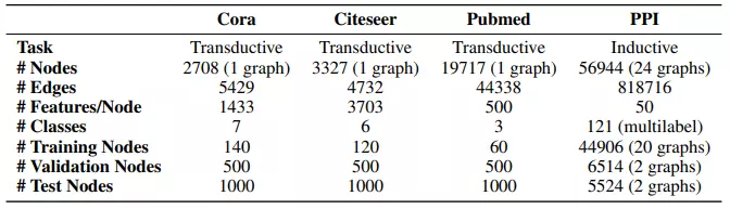
Thông tin về các bộ dữ liệu được sử dụng làm thực nghiệm.
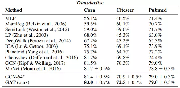
Bảng dưới tổng hợp kết quả cho bài toán phân loại trên 3 tập dữ liệu Cora, Citeseer và Pubmed.
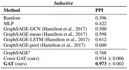
Bảng dưới là tổng hợp F1-score của cá mô hình trên tập dữ liệu PPI.
Tham khảo
[1] Graph Attention Networks, Petar Veličković et al., ICLR 2018
[2] https://github.com/gordicaleksa/pytorch-GAT/tree/main
[3] pytorch-GAT, Gordić, Aleksa
[4] Fake News Detection on Social Media using Geometric Deep Learning, Federico Monti et al
[5] Traffic Prediction with advanced Graph Neural Networks, DeepMind
[6] Spectral Networks and Deep Locally Connected Networks on Graphs, Joan Bruna et al
[8] Inductive Representation Learning on Large Graphs, William L. Hamilton et al., NIPS
[10] Graph attention network - DGL
[11] How to get started with Graph Machine Learning, Gordić, Aleksa
All rights reserved
