Continue with Machine Learning - Image Processing

In this post we take a look at image processing such as image compression using Machine Learning technique.

Image Processing

Image processing is very useful when dealing with large quantity of images. We want image size to be big enough to contain useful information yet small enough for processing speed. Speed, Memory can be very demanding when traing machine learning model. So more than often we need to compress the images to the size that is just good enough to make training model efficient and useful.

The technique used is called vector quantization, one of the technique used in data compression. we compress image by storing fewer bits for the image, that is to decrease the bit-depth of the image. There are more details here to data compression.

Machine learning algorithms used is called KMeans clustering. Loosely speaking, what the algorithm does to the image is choosing many centroids to represent clusters of image pixels. centroid is like the average of a bunch of pixels bits.

OK, let's get to coding. We first import some libraries.

# argparse is for building command line with arguments
import argparse
# numpy for manipulating array
import numpy as np
# scipy misc library is for loading image
from scipy import misc 
# sklearn for machine learning algorithms, 
# here we import cluster algorithms groups 
# which includes KMeans algorithms
from sklearn import cluster
# matplotlib is for plotting
import matplotlib.pyplot as plt

Let make command line parser.

def build_arg_parser():
    parser = argparse.ArgumentParser(description='Compressing the image \
            using clustering')
    parser.add_argument("--input-file", dest="input_file", required=True,
            help="Input image")
    parser.add_argument("--num-bits", dest="num_bits", required=False,
            type=int, help="Number of bits used to represent each pixel")
    return parsers

Then let create function for compressing image using KMeans algorithms.

def compress_image(img, num_clusters):
    # Convert input image into an array of shape (num_samples, num_features)
    # to run kmeans clustering algorithm
    puts img.shape
    X = img.reshape((-1, 1))
    puts img.shape
    # Run kmeans on input data
    kmeans = cluster.KMeans(n_clusters=num_clusters, n_init=4, random_state=5)
    kmeans.fit(X)
    centroids = kmeans.cluster_centers_.squeeze()
    labels = kmeans.labels_

    # Assign each value to the nearest centroid and
    # reshape it to the original image shape
    input_image_compressed = np.choose(labels, centroids).reshape(img.shape)

    return input_image_compressed

Next, we create image plotting function.

def plot_image(img, title):
    vmin = img.min()
    vmax = img.max()
    plt.figure()
    plt.title(title)
    plt.imshow(img, cmap=plt.cm.gray, vmin=vmin, vmax=vmax)

Last, we create main function to run on command line.

if __name__=='__main__':
    args = build_arg_parser().parse_args()
    input_file = args.input_file
    num_bits = args.num_bits

    if not 1 <= num_bits <= 8:
        raise TypeError('Number of bits should be between 1 and 8')

    num_clusters = np.power(2, num_bits)

    # Print compression rate
    compression_rate = round(100 * (8.0 - args.num_bits) / 8.0, 2)
    print('\nThe size of the image will be reduced by a factor of', 8.0/args.num_bits)
    print('\nCompression rate = ' + str(compression_rate) + '%')

    # Load input image
    input_image = misc.imread(input_file, False).astype(np.uint8)
    misc.imsave("compressed.jpg")
    # original image
    plot_image(input_image, 'Original image')

    # compressed image
    input_image_compressed = compress_image(input_image, num_clusters)
    plot_image(input_image_compressed, 'Compressed image; compression rate = '
            + str(compression_rate) + '%')
    misc.imsave("compressed" + str(compression_rate) + "%.png", input_image_compressed)
    plt.show()

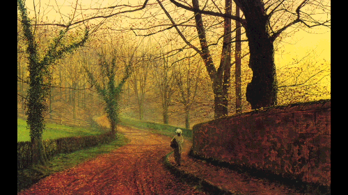
Here is the image with size of 302KB that we are going to compress.

Now let's see the compression in action:

python3 image_compressor.py --input-file red_sky_small.png --num-bits 4

We compress the image to 4 bits by compressing 50%, the image size is 169KB Now let compress it to 2 bits by making it smaller 75%

python3 image_compressor.py --input-file red_sky_small.png --num-bits 2

Now the image size is 64.2KB

Let's do it again to 1 bit by compressing it 87.5%

python3 image_compressor.py --input-file red_sky_small.png --num-bits 1

Now the image size is 28.0KB

See the effect? It's more dramatic in a gray-scale image.

Image size is 60.4KB

Image size is 23.1KB

Image size is 11.2KB

We make gray-scale image by changing the line:

     # Load input image
    input_image = misc.imread(input_file, True).astype(np.uint8) # True here mean gray-scale
    misc.imsave("compressed_gray" + str(compression_rate) + "%.png", input_image_compressed)

I think we can play more with color-map to see the effect of compression. Maybe we can get to know deeper with image processing in the next post.