Đã đăng vào Jun 25th, 2017 2:11 p.m. 5 phút đọc

890

Case Study: Solving Kaggle's Titanic machine learning competition

Bài đăng này đã không được cập nhật trong 2 năm

In my previous article, I wrote about example of using marchine learning algorithms via scikit-learn. However, the Iris dataset dataset has already prepare for learning. In this article, we mainly focus on data preparation before we can fit it into our learning model. What is data preparation?

What is data preparation?

Believe me or not, the machine learning engineer spend 80% of their times for preparing data, and 20% for training and improving the model. The way of machine learning work is simple. It learns from the old data and then it predict the output for a given input base on the previous example. Therefore, it is critical that you feed them the right data for the problem you want to solve. Even if you have good data, you need to make sure that it is in a useful scale, format and even that meaningful features are included.

Why don't we raw data to train our model? why we need to prepare our data? Because not all features in our dataset are nacessary to address the problem, and some features might have missing value, strong in wrong format. When we include those features to our training, it can cause problems to our generalization. So we need to process those field first.

In this post we are going to use titanic dataset train.csv from Kaggle. Because it is a raw data, so we need to prepare first.

Data Preparation Process

There are three for data preparation:

Select Data
Process Data
Transform Data

To learn more about the definition of data preparation click here

First of all, we will use some libraries: sklearn for machine learnig algorithms, pandas, numpy for handling the data, and seaborn, matplotlib for our data visualization

# data analysis and wrangling
import pandas as pd
import numpy as np
import random as rnd

# visualization
import seaborn as sns
import matplotlib.pyplot as plt

# machine learning
from sklearn.model_selection import StratifiedShuffleSplit
from sklearn.metrics import accuracy_score, log_loss
from sklearn.linear_model import LogisticRegression
from sklearn.svm import SVC, LinearSVC
from sklearn.ensemble import RandomForestClassifier
from sklearn.neighbors import KNeighborsClassifier
from sklearn.naive_bayes import GaussianNB
from sklearn.linear_model import Perceptron
from sklearn.linear_model import SGDClassifier
from sklearn.tree import DecisionTreeClassifier

Now, let's start prepare our titanic dataset and learn from it.

1. Select Data and Processs Data

Select Data: is concerned with selecting the subset of all available data that you will be working with. The process of selecting data are used to identify the relevant and irrelevant feature. Preprocess Data: After you have selected the data, you need to consider how you are going to use the data. This preprocessing step is about getting the selected data into a form that you can work. Three common data preprocessing steps are formatting, cleaning and sampling.

First, we need read our dataset, and try to understand the given information from data itself.

train_df = pd.read_csv('train.csv')
print(train_df.columns.values)
#['PassengerId' 'Survived' 'Pclass' 'Name' 'Sex' 'Age' 'SibSp' 'Parch'  'Ticket' 'Fare' 'Cabin' 'Embarked']

train_df.info()
#<class 'pandas.core.frame.DataFrame'>
#RangeIndex: 891 entries, 0 to 890
#Data columns (total 12 columns):
#PassengerId    891 non-null int64
#Survived       891 non-null int64
#Pclass         891 non-null int64
#Name           891 non-null object
#Sex            891 non-null object
#Age            714 non-null float64
#SibSp          891 non-null int64
#Parch          891 non-null int64
#Ticket         891 non-null object
#Fare           891 non-null float64
#Cabin          204 non-null object
#Embarked       889 non-null object
#dtypes: float64(2), int64(5), object(5)
#memory usage: 83.6+ KB

Let's preview our data

print(train_df.head())
#PassengerId	Survived	Pclass	Name	Sex	Age	SibSp	Parch	Ticket	Fare	Cabin	Embarked
#1	0	3	Braund, Mr. Owen Harris	male	22.0	1	0	A/5 21171	7.2500	NaN	S
#2	1	1	Cumings, Mrs. John Bradley (Florence Briggs Th...	female	38.0	1	0	PC 17599	71.2833	C85	C
#3	1	3	Heikkinen, Miss. Laina	female	26.0	0	0	STON/O2. 3101282	7.9250	NaN	S
#4	1	1	Futrelle, Mrs. Jacques Heath (Lily May Peel)	female	35.0	1	0	113803	53.1000	C123	S
#5	0	3	Allen, Mr. William Henry	male	35.0	0	0	373450	8.0500	NaN	S

print(train_df.tail())
#PassengerId	Survived	Pclass	Name	Sex	Age	SibSp	Parch	Ticket	Fare	Cabin	Embarked
#887	0	2	Montvila, Rev. Juozas	male	27.0	0	0	211536	13.00	NaN	S
#888	1	1	Graham, Miss. Margaret Edith	female	19.0	0	0	112053	30.00	B42	S
#889	0	3	Johnston, Miss. Catherine Helen "Carrie"	female	NaN	1	2	W./C. 6607	23.45	NaN	S
#890	1	1	Behr, Mr. Karl Howell	male	26.0	0	0	111369	30.00	C148	C
#891	0	3	Dooley, Mr. Patrick	male	32.0	0	0	370376	7.75	NaN	Q

Now, let's investigate our features one by one:

Pclass:

print(train_df[['Pclass', 'Survived']].groupby(['Pclass']).mean())
#Pclass  Survived
#1       0.629630
#2       0.472826
#3       0.242363

As you can see this feature has some impact to the output. So we keep it

Name: because name has no association survival chance, so we do not need it.

Sex:

print(train_df[['Sex', 'Survived']].groupby(['Sex']).mean())
#Sex        Survived
#female  0.742038
#male    0.188908

Base on information above, we saw that weman has a survival chance high, so we need this feature for our learning.

Age: We have some missing values in this feature. Since it a number we can fill the missing value from a random number between (mean -std) and (mean + std), and we categorize age into 5 range.

 for dataset in full_data:
 age_avg = dataset['Age'].mean()
 age_std  = dataset['Age'].std()

 dataset['Age'] = dataset['Age'].fillna(np.random.randint(age_avg - age_std, age_avg + age_std))
 dataset['Age'] = dataset['Age'].astype(int)

  print(train_df['Age'].describe())
  #count    891.000000
  #mean      31.928171
  #std       13.773505
  #min        0.000000
  #25%       22.000000
  #50%       32.000000
  #75%       41.000000
  #max       80.000000
  #Name: Age, dtype: float64

train_df['CategoricalAge'] = pd.cut(train_df['Age'], 5)
print(train_df[['CategoricalAge', 'Survived']].groupby(['CategoricalAge']).mean())
#CategoricalAge  Survived
#(-0.08, 16.0]   0.550000
#(16.0, 32.0]    0.370690
#(32.0, 48.0]    0.349862
#(48.0, 64.0]    0.434783
#(64.0, 80.0]    0.090909

SibSp and Parch: With the number of siblings/spouse and the number of children/prarents we can create a new feature class Family Size.

for dataset in full_data:
    dataset['FamilySize'] = dataset['SibSp'] + dataset['Parch'] + 1

print(train_df[['FamilySize', 'Survived']].groupby(['FamilySize']).mean())
#FamilySize     Survived
#1           0.303538
#2           0.552795
#3           0.578431
#4           0.724138
#5           0.200000
#6           0.136364
#7           0.333333
#8           0.000000
#11          0.000000

#  Let check whether they are alone in the ship or not.
for dataset in full_data:
    dataset['IsAlone'] = 0
    dataset.loc[dataset['FamilySize'] == 1, 'IsAlone'] = 1
print(train_df[['IsAlone', 'Survived']].groupby(['IsAlone']).mean())
#IsAlone     Survived
#0        0.505650
#1        0.303538

Ticket: The change of survive is not depent on ticket number, so we no need this feature.

Fare: There is some missing value in these feature, and we will replace it with the median. Then we can categorize it into 4 ranges.

for dataset in full_data:
dataset['Fare'] = dataset['Fare'].fillna(dataset['Fare'].median())

train_df['CategoricalFare'] = pd.qcut(train_df['Fare'], 4)
print(train_df[['CategoricalFare', 'Survived']].groupby(['CategoricalFare']).mean())
#CategoricalFare     Survived
#(-0.001, 7.91]   0.197309
#(7.91, 14.454]   0.303571
#(14.454, 31.0]   0.454955
#(31.0, 512.329]  0.581081

Cabin: The cabin number cannot determine the survival chance, so we do not need to feature.

Embarked: There is some missing value in these feature, and we will fill with the most occurred value in this feature ('S).

for dataset in full_data:
    dataset['Embarked'] = dataset['Embarked'].fillna('S')
print(train_df[['Embarked', 'Survived']].groupby(['Embarked']).mean())
#Embarked    Survived
#C         0.553571
#Q         0.389610
#S         0.339009

3. Transform Data

Transform data is the process transformations our dataset's feature into format where machine can learn from. This step is also referred to as feature engineering. Let's transform our dataset's features:

for dataset in full_data:
    # Mapping Sex
    dataset['Sex'] = dataset['Sex'].map({'female': 0, 'male': 1}).astype(int)
    
    # Mapping Embarked
    dataset['Embarked'] = dataset['Embarked'].map({'S': 0, 'C': 1, 'Q': 2}).astype(int)
    
    # Mapping Fare
    dataset.loc[dataset['Fare'] <= 7.91, 'Fare'] = 0
    dataset.loc[(dataset['Fare'] > 7.91) & (dataset['Fare'] <= 14.454), 'Fare'] = 1
    dataset.loc[(dataset['Fare'] > 14.454) & (dataset['Fare'] <= 31), 'Fare'] = 2
    dataset.loc[dataset['Fare'] > 31, 'Fare'] = 3
    dataset['Fare'] = dataset['Fare'].astype(int)
    
    # Mapping Age
    dataset.loc[ dataset['Age'] <= 16, 'Age']  = 0
    dataset.loc[(dataset['Age'] > 16) & (dataset['Age'] <= 32), 'Age'] = 1
    dataset.loc[(dataset['Age'] > 32) & (dataset['Age'] <= 48), 'Age'] = 2
    dataset.loc[(dataset['Age'] > 48) & (dataset['Age'] <= 64), 'Age'] = 3
    dataset.loc[ dataset['Age'] > 64, 'Age'] = 4
    dataset['Age'] = dataset['Age'].astype(int)
    
# Feature Selection: remove unnacessary field
drop_features = ['PassengerId', 'Name', 'Ticket', 'Cabin', 'SibSp', 'Parch', 'FamilySize']
train_df = train_df.drop(drop_features, axis=1)
train_df = train_df.drop(['CategoricalAge', 'CategoricalFare'], axis=1)
    
test_df_droped = test_df.drop(drop_features, axis = 1)
trainingSet = train_df.values
testingSet  = test_df_droped.values

# let print the sample of our final prcessing
print (train_df.head(10))

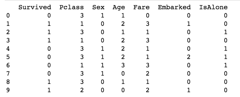
Here, we got the dataset where we can fit into our learning model, and it's time to train our learning model.

Apply Learning Algorithms

After finish preparing our data, it's time to apply learning algorithms to train our model same as what we did in previous post.

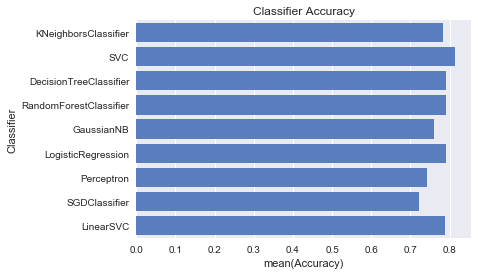
# Classifier Comparision
classifiers = [
    KNeighborsClassifier(3),
    SVC(probability=True),
    DecisionTreeClassifier(),
    RandomForestClassifier(),
    GaussianNB(),
    LogisticRegression(),
    Perceptron(),
    SGDClassifier(),
    LinearSVC()
]

log_cols = ["Classifier", "Accuracy"]
log = pd.DataFrame(columns=log_cols)
sss = StratifiedShuffleSplit(n_splits=10, test_size=0.1, random_state=0)
X = trainingSet[0::, 1::]
y = trainingSet[0::, 0]

acc_dict = {}
for train_index, test_index in sss.split(X,y):
    X_train, X_test = X[train_index], X[test_index]
    y_train, y_test = y[train_index], y[test_index]
    
    for clf in classifiers:
        name = clf.__class__.__name__
        clf.fit(X_train, y_train)
        train_predictions = clf.predict(X_test)
        acc = accuracy_score(y_test, train_predictions)
        if name in acc_dict:
            acc_dict[name] += acc
        else:
            acc_dict[name] = acc

for clf in acc_dict:
    acc_dict[clf] = acc_dict[clf] / 10.0
    log_entry = pd.DataFrame([[clf, acc_dict[clf]]], columns=log_cols)
    log = log.append(log_entry)
    
plt.xlabel('Accuracy')
plt.title('Classifier Accuracy')

sns.set_color_codes("muted")
sns.barplot(x='Accuracy', y='Classifier', data=log, color='b')

And here we got:

Let's predict the given test data and submit the result to kaggle.

model = SVC(probability=True)
model.fit(X, y)
Y_pred = model.predict(testingSet)

submission = pd.DataFrame({
     "PassengerId": test_df["PassengerId"],
     "Survived": Y_pred
 })
submission
submission.to_csv('submission.csv', index=False)

And here the result:

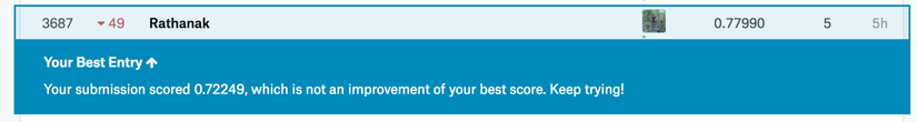
0.77 or 77% not bad, but it not goot enough. With your help on preparing the data we might able improve it, so please put your suggestion in comment belove.

Resources

Summary

The key to has a good modeling is to has a good data, and it still better even your learning algorithms is not so good. Therefore, getting good at data preparation will make you a master at machine learning. However, to master the data preparation you need to do a lot of iterations of exploration and analysis. And for data preparing above, if you have any suggestion to improve it please put the comment belove.

Machine Learning Python