Into to Machine Learning: Practical supervised learning algorithms with Scikit-learn
Bài đăng này đã không được cập nhật trong 2 năm
 In the coding on my previous post Into to Machine Learning: Supervised learning, I showed you about supervised learning. In the code example, I showed an example using
 scikit-learn library. In this post, I am going show you examples of applying supervised learning algorithm to generalize the data with ease via scikit-learn. But, what is scikit-learn? and why I choose scikit-learn for these demonstration?
What/why is scikit-learn?
Started in 2007 by David Cournapeau as a Google Summer of Code project, scikit-learn is a Python module for machine learning built on top of SciPy and distributed under the 3-Clause BSD license. The reason which I choose scikit-learn because it is easy for beginner to get up and running with the popular machine learning algorithm, and it also has famous built-in Iris dataset which we can play along.
Sample dataset
The dataset which we use in post is Iris Dataset. This datasets consists of 3 different types of irises' (Setosa, Versicolour, and Virginica) petal and sepal length and 50 sample for each type(150 in total) . Each array item store the sample measurements: sepal length, sepal width, petal length, and petal width. I choose Iris dataset because:
- Famous dataset for machine learning because prediction is easy
- Framed as a supervised learning problem: Predict the species of an iris using the measurements
- It already come with scikit-learn
For more detail about the dataset visit: http://archive.ics.uci.edu/ml/datasets/Iris.
Let's load and test the
Iris Dataset:
# import load_iris function from datasets module
from sklearn.datasets import load_iris

# store dataset in variable iris
iris = load_iris()

print(iris.data.shape)
# (150, 4)

# show the name of featues
print(iris.feature_names)
#  ['sepal length (cm)', 'sepal width (cm)', 'petal length (cm)', 'petal width (cm)']
Awesome, now let's apply supervised learning algorithms on this data.
Supervised Algorithms
1. Naive Bayes
The Naive Bayesian classifier is based on Bayes’ theorem with independence assumptions between predictors.
from sklearn.datasets import load_iris
from sklearn.model_selection import train_test_split
from sklearn import metrics
from sklearn.naive_bayes import GaussianNB
# read in the iris data
iris = load_iris()

# create X (features) and y (label)
X = iris.data
y = iris.target

# use train/test split with different random_state values
X_train, X_test, y_train, y_test = train_test_split(X, y, random_state=4)

clf = GaussianNB()
clf.fit(X_train, y_train)
# GaussianNB(priors=None)

# predict our sample
y_pred = model.predict(X_test)

# evaluation our prediction
print(metrics.accuracy_score(y_test, y_pred))
# 0.973684210526
Result: 0.973684210526 of accuracy. To learn more about Naive Bayes:
- http://scikit-learn.org/stable/modules/generated/sklearn.naive_bayes.GaussianNB.html#sklearn.naive_bayes.GaussianNB
- http://scikit-learn.org/stable/modules/naive_bayes.html#naive-bayes
- https://en.wikipedia.org/wiki/Naive_Bayes_classifier
- https://www.youtube.com/watch?v=ICKBWIkfeJ8&list=PLAwxTw4SYaPkQXg8TkVdIvYv4HfLG7SiH
- http://machinelearningmastery.com/naive-bayes-for-machine-learning/
2. Support Vector Machines
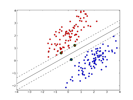 Support Vector Machines (SVM) are a method that uses points in a transformed problem space that best separate classes into two groups. Classification for multiple classes is supported by a one-vs-all method. SVM also supports regression by modeling the function with a minimum amount of allowable error.
from sklearn.datasets import load_iris
from sklearn.model_selection import train_test_split
from sklearn import metrics
from sklearn.svm import SVC

# read in the iris data
iris = load_iris()

# create X (features) and y (label)
X = iris.data
y = iris.target

# use train/test split with different random_state values
X_train, X_test, y_train, y_test = train_test_split(X, y, random_state=4)

svm = SVC()
svm.fit(X_train,y_train)
# SVC(C=1.0, cache_size=200, class_weight=None, coef0=0.0,
#   decision_function_shape=None, degree=3, gamma='auto', kernel='rbf',
#   max_iter=-1, probability=False, random_state=None, shrinking=True,
#   tol=0.001, verbose=False)

# predict our sample
y_pred = scv.predict(X_test)

# evaluation our prediction
print(metrics.accuracy_score(y_test, y_pred))
# 0.973684210526
Result: 0.973684210526 of accuracy.
To learn more about Support Vector Machines:
- http://scikit-learn.org/stable/modules/generated/sklearn.svm.SVC.html#sklearn.svm.SVC
- http://scikit-learn.org/stable/modules/svm.html#svm
- https://en.wikipedia.org/wiki/Support_vector_machine
- https://www.youtube.com/watch?v=ICKBWIkfeJ8&list=PLAwxTw4SYaPkQXg8TkVdIvYv4HfLG7SiH
3. DecisionTree
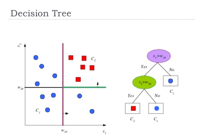 Classification and Regression Trees or CART for short is a term introduced by Leo Breiman to refer to Decision Tree algorithms that can used for classification or regression predictive modeling problems. It breaks down a dataset into smaller and smaller subsets, and the final result is a tree with decision nodes and leaf nodes where leaf nodes are the label(respond).
from sklearn.datasets import load_iris
from sklearn.model_selection import train_test_split
from sklearn import metrics
from sklearn.tree import DecisionTreeClassifier

# read in the iris data
iris = load_iris()

# create X (features) and y (label)
X = iris.data
y = iris.target

# use train/test split with different random_state values
X_train, X_test, y_train, y_test = train_test_split(X, y, random_state=4)

tree = DecisionTreeClassifier()
tree.fit(X_train,y_train)
# DecisionTreeClassifier(class_weight=None, criterion='gini', max_depth=None,
#            max_features=None, max_leaf_nodes=None,
#            min_impurity_split=1e-07, min_samples_leaf=1,
#            min_samples_split=2, min_weight_fraction_leaf=0.0,
#            presort=False, random_state=None, splitter='best')

# predict our sample
y_pred = tree.predict(X_test)

# evaluation our prediction
print(metrics.accuracy_score(y_test, y_pred))
# 0.973684210526
Result: 0.973684210526 of accuracy. To learn more about DecisionTree:
- http://scikit-learn.org/stable/modules/tree.html#tree
- http://scikit-learn.org/stable/modules/generated/sklearn.tree.DecisionTreeClassifier.html#sklearn.tree.DecisionTreeClassifier
- https://en.wikipedia.org/wiki/Decision_tree_learning
- http://machinelearningmastery.com/classification-and-regression-trees-for-machine-learning/
- https://www.youtube.com/watch?v=ICKBWIkfeJ8&list=PLAwxTw4SYaPkQXg8TkVdIvYv4HfLG7SiH
4. Logistic Regression
Logistic regression makes predictions on data by take any real input and the output always takes values between zero and one.
from sklearn.datasets import load_iris
from sklearn.model_selection import train_test_split
from sklearn import metrics
from sklearn.linear_model import LogisticRegression

# read in the iris data
iris = load_iris()

# create X (features) and y (label)
X = iris.data
y = iris.target

# use train/test split with different random_state values
X_train, X_test, y_train, y_test = train_test_split(X, y, random_state=4)

logistic_model = LogisticRegression()
logistic_model.fit(X_train, y_train)
# LogisticRegression(C=1.0, class_weight=None, dual=False, fit_intercept=True,
#          intercept_scaling=1, max_iter=100, multi_class='ovr', n_jobs=1,
#          penalty='l2', random_state=None, solver='liblinear', tol=0.0001,
#          verbose=0, warm_start=False)

# predict our sample
y_pred = logistic_model.predict(X_test)

# evaluation our prediction
print(metrics.accuracy_score(y_test, y_pred))
# 0.921052631579
Result: 0.921052631579 of accuracy. To learn more about Logistic Regression:
- http://scikit-learn.org/stable/modules/generated/sklearn.linear_model.LogisticRegression.html
- https://en.wikipedia.org/wiki/Logistic_regression
5. k-Nearest Neighbor
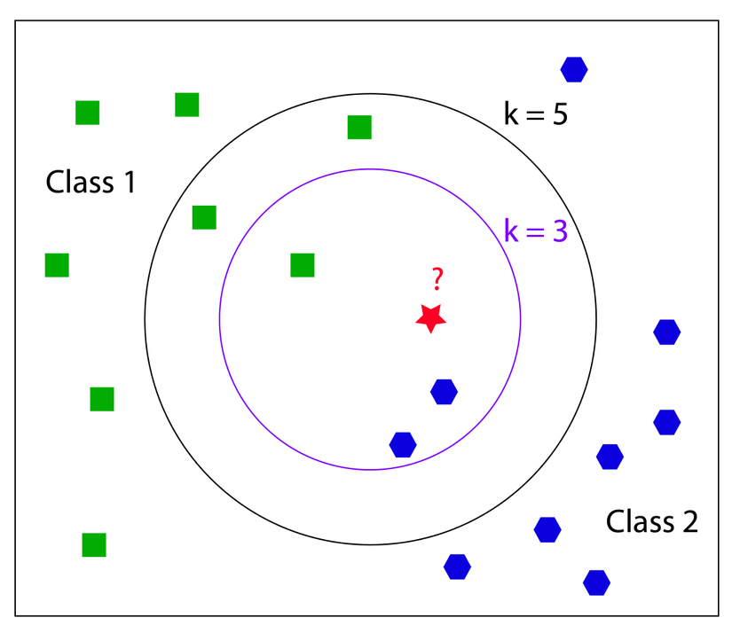 The k-Nearest Neighbor (kNN) algorithm makes predictions by locating similar cases to a given data instance (using a similarity function) and returning the average or majority of the most similar data instances. The kNN algorithm can be used for classification or regression.
from sklearn.datasets import load_iris
from sklearn.model_selection import train_test_split
from sklearn import metrics
from sklearn.neighbors import KNeighborsClassifier

# read in the iris data
iris = load_iris()

# create X (features) and y (label)
X = iris.data
y = iris.target

# use train/test split with different random_state values
X_train, X_test, y_train, y_test = train_test_split(X, y, random_state=3)

# check classification accuracy of KNN with K=2
knn = KNeighborsClassifier(n_neighbors=2)
knn.fit(X_train, y_train)
# KNeighborsClassifier(algorithm='auto', leaf_size=30, metric='minkowski',
#          metric_params=None, n_jobs=1, n_neighbors=2, p=2,
#           weights='uniform')

# predict our sample
y_pred = knn.predict(X_test)

# evaluation our prediction
print(metrics.accuracy_score(y_test, y_pred))
# 0.947368421053

# Let do it agian with difference random_state and K
# use train/test split with different random_state values
X_train, X_test, y_train, y_test = train_test_split(X, y, random_state=4)

# check classification accuracy of KNN with K=5
knn = KNeighborsClassifier(n_neighbors=5)
knn.fit(X_train, y_train)
# KNeighborsClassifier(algorithm='auto', leaf_size=30, metric='minkowski',
#           metric_params=None, n_jobs=1, n_neighbors=5, p=2,
#           weights='uniform')

# predict our sample
y_pred = knn.predict(X_test)

# evaluation our prediction
print(metrics.accuracy_score(y_test, y_pred))
# 0.947368421053
Result:
- 0.947368421053 of accuracy when K = 2, and random_state=3
- 0.947368421053 of accuracy when K = 5, and random_state=4 To learn more about k-Nearest Neighbor:
- http://scikit-learn.org/stable/modules/generated/sklearn.neighbors.KNeighborsClassifier.html#sklearn.neighbors.KNeighborsClassifier
- http://scikit-learn.org/stable/modules/neighbors.html#neighbors
- https://www.youtube.com/watch?v=UqYde-LULfs
- https://www.youtube.com/watch?v=ICKBWIkfeJ8&list=PLAwxTw4SYaPkQXg8TkVdIvYv4HfLG7SiH
Resources
- http://scikit-learn.org/stable/index.html
- https://www.youtube.com/watch?list=PL5-da3qGB5ICeMbQuqbbCOQWcS6OYBr5A&v=elojMnjn4kk
- http://archive.ics.uci.edu/ml/datasets/Iris
- https://en.wikipedia.org/wiki/Iris_flower_data_set
- https://www.youtube.com/watch?v=ICKBWIkfeJ8&list=PLAwxTw4SYaPkQXg8TkVdIvYv4HfLG7SiH
Final Word
In this post, I've shown you a demonstration of applying the most popular and powerful supervied algorithms via scikit-learn for predicting. I hope one of them might help you to solve your problem. However, choosing the right algorithms for your specific problem and tuning its parameters might be tough. And by practicing, you can tell which algorithm is suitable for your problems.
So, stop reading and let's start typing.
All rights reserved
