Linear Regression with One Variable

Bài đăng này đã không được cập nhật trong 2 năm

You see anything interesting in the tech world is implicitely or explicitely related to machine learning. From finding contacts through voice in nokia phone to modern day facebook suggestions, almost everything is based on concept of machine learning. So we will learn some overview of machine learning first.

Machine Learning:

Machine learning is a subpart of computer science that learns pattern from set of data and then try to predict output from similiar data. It is like language learning of new born child. A child learn how to utter a letter by seeing and practicing with superiors. that means they are trained for years and years and thus achieve perfection. Machine learning techniques are best to use when you cannot code the rules and also you cannot scale. Some populer machine learning techniques are:

Supervised Learning: Supervised learning algorithms are trained using labeled examples, such as an input where the desired output is known. The learning algorithm receives a set of inputs along with the corresponding correct outputs, and the algorithm learns by comparing its actual output with correct outputs to find errors. It then modifies the model accordingly.
Unsupervised learning: Unsupervised learning is used against data that has no historical labels. The system is not told the "right answer." The algorithm must figure out what is being shown. The goal is to explore the data and find some structure within. Unsupervised learning works well on transactional data.

Linear Regression with One Variable

Linear regression with one variable is also known as "univariate linear regression". In regression problems, we taking input variables and trying to fit the output onto acontinuous expected result function. Univariate linear regression is used when you want to predict a single output value from a single input value. We now introduce notation for equations

m=number of training examples x′s=input variable/features y′s=output variable/target variable (x,y)=one training example (x(i),y(i))=ith training example

now we see the model representation:

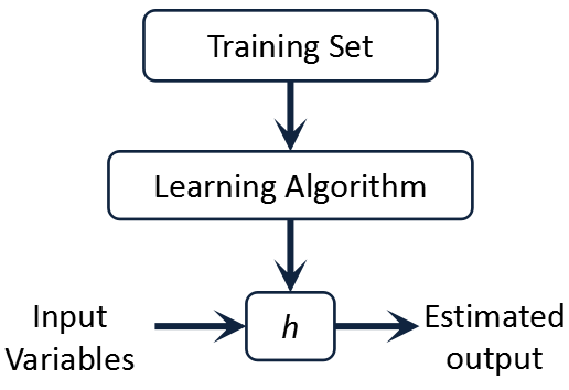
so from the image, we give training set to learning algorithm. After eating training set the learning algorithm creates which by convention is usually denoted lowercase h and h stands for hypothesis. And hypothesis is a function that maps from x's to y's.

The Hypothesis Function

There are many tipes of hypothesis function. But we take the general hθ(x)=θ0+θ1x You can simply realise that it is similiar to the y=mx+c. so θ1 is the slope of line. We give to hθ(x) values for θ0 and θ1 to get our output y. In other words, we are trying to create a function called hθ that is trying to map our input data (the x's) to our output data (the y's).

Example:

we can make a random guess about our hθ function: θ0=2 and θ1=2. The hypothesis function becomes hθ(x)=2+2x.

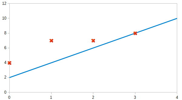
The red crosses indicate y's and the blue line is our hypothesis.

So for input of 1 to our hypothesis, y will be 4. This is off by 3. Note that we will be trying out various values of θ0 and θ1 to try to find values which provide the best possible "fit" or the most representative "straight line" through the data points mapped on the x-y plane.

Cost Function

We can measure the accuracy of our hypothesis function by using a cost function. This takes an average of all the results of the hypothesis with inputs from x's compared to the actual output y's.

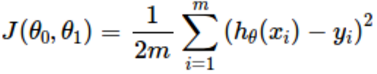
This function is called mean squared error. This mean is halved as a ease of computing gradient descent, as the derivative term of the square function will cancel out the 1/2 term.

Cost Function Intuition

We start with simple hypothesis hθ=θ1x. After plotting graph of parameter vs cost function, we will get something like this

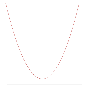
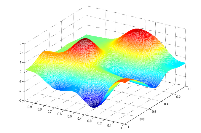
so our main target is to find the local minima for that curve. That means for parameter on that least point error is also minimum. The same can be done for higher level of degree for hypothesis function. Eventually we will get something like this