Let's learn Octave

I run across an unpopular yet powerful language called Octave. If you know Matlab, Octave won't be a terrible language to catch on.

The most attractive feature of Octave is its well-written, robust library on matrix manipulations. The word matrix might sound obscure or scary to some, but matrix is just an array of elements arranged in rows and columns. What do we use matrix for? High performance and ease to use of massive data used in statistics, data science and machine learning, to list a few.

Installation

Let's install and make it run. Octave can be used on Windows and Linux. Here I use Linux.

sudo apt-get update
sudo apt-get install octave

This is a version with GUI. by the time of my writing, Octave has already come out with version 4.0.2. We can run with GUI or terminal. Here we demonstrate by using terminal.

octave #run with GUI
octave-cli # run without GUI

Let's run

In this post I try my best to show the strength of Octave. Mind you, that Octave can do almost other language, such ruby and python can do, but it shift its main focus on numerical computations and data visualization and manipulation.

Let's get into the business!

Basic Operations

3 + 4  %=> 7
4 * 5  %=> 20

2 == 3 %=> 0 means false

2 ~= 3 %=> 1 means true

1 && 0 %=> 0

1 && 0 %=> 1

Note that '%' is used to start comments.

If you don't want to see long prompt such as 'octave-1', you can change it with ```PS1('>> ').

One more thing to note is that you can end a statement with or with a semicolon ;. If you don't put semicolon, the output will display, otherwise it will not.

You can assign a variable:

 a = 1

 c = pi %=> 3.1416

 d = (pi > 3)

You can display with disp.

  disp(d); %=> 1
  disp(sprintf('5 decimals: %0.5f', c)) % 5 decimals: 3.14159

This is similar to C language format.

You can change format to short and long decimal place:

format long
c %=> c = 3.14159265358979
format short
c %=> c = 3.1416

Let's go into the core of Octave Matrix

X = [1 2; 3 4; 5 6]
% X =
  1  2
  3  4
  5  6

semicolon ';' is to mark the end of a row. X is a 3 by 2 matrix.

v = [4 5 6]
% v =
  4  5  6

v is a 1-by-3 vector.

But if v = [4; 5; 6] % v = 1 2 3

v is 3-by-1 vector.

we generate vector and matrix as below:

v = 1:5
% v =
  1  2  3  4  5  6

c =  ones(3, 2)
% c =
 1  1
 1  1
 1  1

This is the same as writing:

c = [1 1;1 1;1 1]
% c =
 1  1
 1  1
 1  1

And also

c = zeros(2, 3)
% c =
 0 0 0
 0 0 0

Or get some random number between 0 and 1

c = rand(2, 3)
% c =
  0.91366   0.78837   0.24759
  0.95977   0.20207   0.60540

Below is identity matrix:

eye(4)
ans =
Diagonal Matrix
1  0  0
0  1  0
0  0  1

Graphics and Manipulation of big data

You can access directory with octave terminal

pwd
% ans = /home/chivorn

'ls' list all the files and directories 'cd' change directory

suppose we have a data file data.dat we can load the data:

load 'data.dat'
who  % show the current variables such as 'a', 'ans' and 'data'...
data % will show all the data
data =

   0.580798   0.254872
   0.469875   0.166915
   0.635548   0.688823
   0.130228   0.876621
   0.714885   0.496422
   0.519935   0.205334
   0.160221   0.871987
   0.075342   0.584289
   ...
   ...
   ...

Let's save

v = data(1:10,:) % this means get the first 10 row
save ten.mat v; % Save v to file 'ten.mat'

You will see the file in current directory

clear % will clear all the current variables

You can select rows
```Octave

C=v([2,4],:)
%
ans =
0.469875   0.166915
0.130228   0.876621

Get 2 and 4 row. Note Octave begin with index 1, not 0. You add row or column to existing matrix.

C = [ones(2,1), C]  %Add one row to the left
C =
1  0.469875  0.166915
1  0.130228  0.876621

Combine matrix together

A = [1 2; 3 4; 5 6];
B = [7 8; 9 10; 11 12];
C = [A B]
C =
 1    2    7    8
 3    4    9   10
 5    6   11   12
D = [A ; B]
D =
    1    2
    3    4
    5    6
    7    8
    9   10
   11   12
size(C)
ans =
  3  4
size(D)
ans =
  2  6

Element-wise operations

E = A .* B
E =

    7   16
   27   40
   55   72
F = A .+ B
F =
    8   10
   12   14
   16   18

G = log(A) * natural log function
G =
   0.00000   0.69315
   1.09861   1.38629
   1.60944   1.79176

Transpose of a matrix

H = A'
ans =
   1   3   5
   2   4   6

Min and Max function also work magically

max(A) % compare maximum along a column
ans =
  5  6

And inverse function

E = magic(3) % return magic square matrix
I = pinv(E)
I =
   0.147222  -0.144444   0.063889
  -0.061111   0.022222   0.105556
  -0.019444   0.188889  -0.102778

Plot data

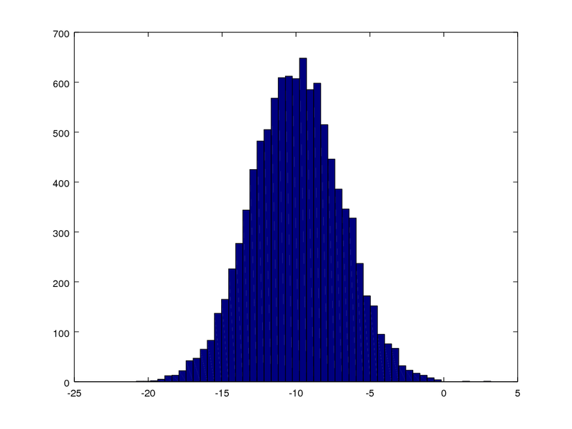
Let's plot a histogram of some random number

w = -10 + 3 * randn(1,10000)  % create a random number
hist(w, 50)  % plot a histogram
print -dpng 'myPlot.png'  % save graph

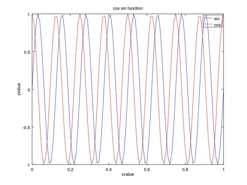
Let's plot one more function.

t=[0:0.01:1]
y =  sin(2*pi*8*t);
plot(t,y)
z = cos(2*pi*8*t);
hold on;
plot(t,z,'r')
legend('sin', 'cos');
xlabel('xvalue');
ylabel('yvalue');
title('cos sin function');
print -dpng 'wave.png'

Still a lot of features and functions to explore. Hope you get some idea about what Octave is. Powerful creature!