Gradient descent - Optimazation algorithm

Hello every body ^^, Have you ever heard about optimazation problem in predictor of machine learning? Before taking about that, we glide example below:

An example of spam email classification

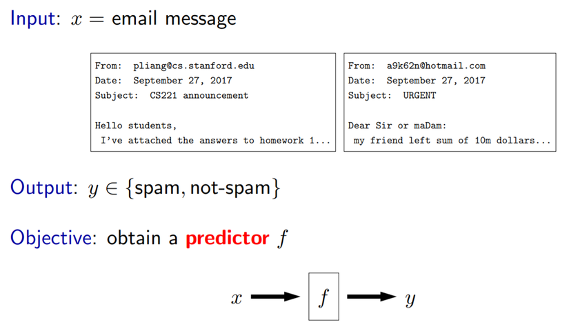First, some terminology. A predictor is a function f that maps an input x to an output y. In statistics, y is known as a response, and when x is a real vector, then it is known as the covariates. The starting point of machine learning is the data, which is the main resource that we can use to address the information complexity of the prediction task at hand. In the post, we will focus on supervised learning, in which our data provides both inputs and outputs, in contrast to unsupervised learning, which only provides inputs. A (supervised) example (also called a data point or instance) is simply an input-output pair (x, y), which specifies that y is the ground-truth output for x. The training data Dtrain is a multiset of examples (repeats are allowed, but this is not important), which forms a partial specification of desired behavior of the predictor. One question released that How to separate email into spam or not??? It is based on Feature extraction: Given input x, output a set of (feature name, feature value) pairs. Example for email classification: 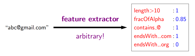We will consider predictors f based on feature extractors. Feature extraction is a bit of an art that requires intuition about both the task and also what machine learning algorithms are capable of. The general principle is that features should represent properties of x which might be relevant for predicting y. It is okay to add features which turn out to be irrelevant, since the learning algorithm can sort it out (though it might require more data to do so). From feature extractor, we have a feature vector of input x: $\phi (x) = \begin{bmatrix} \phi _{1}(x)& \cdot \cdot \cdot & \phi _{d}(x) \\ \end{bmatrix}$ Think of $\phi (x) \epsilon R^{d}$ as a point in a high-dimensional space. For each feature j of feature extraction, we have real number wj representing contribution of feature to prediction 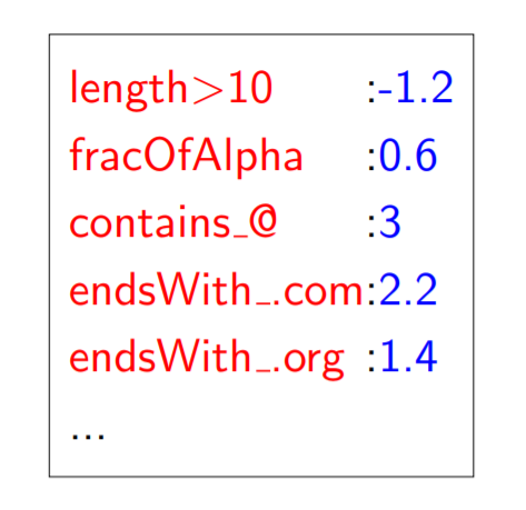We have vector input x, and its weight, we can use predictor to classify data.

Loss function in linear regression

According to above example, we use predictor f_{w} to classsify data (binary classification). But right now, we focus on linear regression. All predictors are whether true or false, and we can trust it in certain percentage. So we have to find a function which denote training error, is loss function. There are some loss function in linear regression such as squared loss , absolute deviation loss. A popular and convenient loss function to use in linear regression is the squared loss, which penalizes the residual of the prediction quadratically. An alternative to the squared loss is the absolute deviation loss, which simply takes the absolute value of the residual. 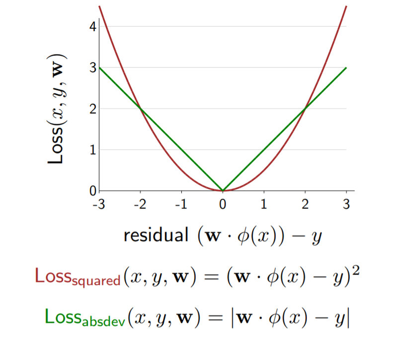Now, look at the formula: $\left ( w \cdot \phi(x)\right ) - y$ is the residual that the amount by which prediction $f_{w} = w\cdot \phi (x)$ overshoots the target y. So if the value of loss function is minimization, our predictor is reliable. One question released: How to minimize loss function ??? Yeah, the scientist has just said that we can find to minimize the TrainLoss(w): 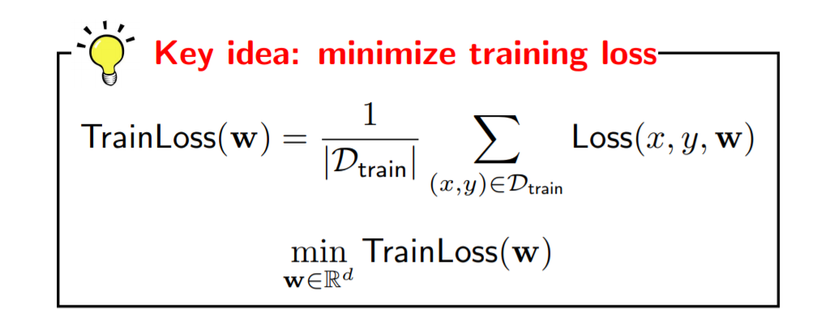So the key that we need to set w to make global tradeoffs — not every example can be happy. This idea urge us to find a optimazation algorithm that minimize TrainLoss(w). It is gradient descent (GD), we will talk about it in below section.

Gradient Descent (GD)

Do not let you wait for long, we are talking about GD right now!. The first, we talk about some concept.

• Gradient: The gradient ∇wTrainLoss(w) is the direction that increases the loss the most.
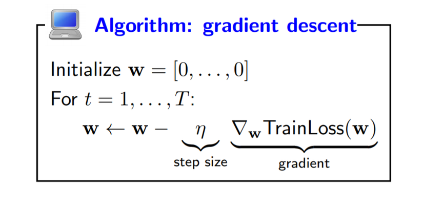
• Descent: So, you can see about above image. A general approach is to use iterative optimization, which essentially starts at some starting point w (say, all zeros), and tries to tweak w so that the objective function value decreases. To do this, we will rely on the gradient of the function, which tells us which direction to move in to decrease the objective the most. The gradient is a valuable piece of information, especially since we will often be optimizing in high dimensions (d on the order of thousands). This iterative optimization procedure is called gradient descent. Gradient descent has two hyperparameters, the step size η (which specifies how aggressively we want to pursue a direction) and the number of iterations T. Let’s not worry about how to set them, but you can think of T = 100 and η = 0.1 for now. Ok, I have just explained the GD 's mean and operation mechanism. As we seen, we have multiple loops before converging. So which loss function is choosen for now ??? In popular, we usually use the squared loss function. Because we can easily direct to move into decrease the objective the most. So in this topic, we focus on least squares regression: 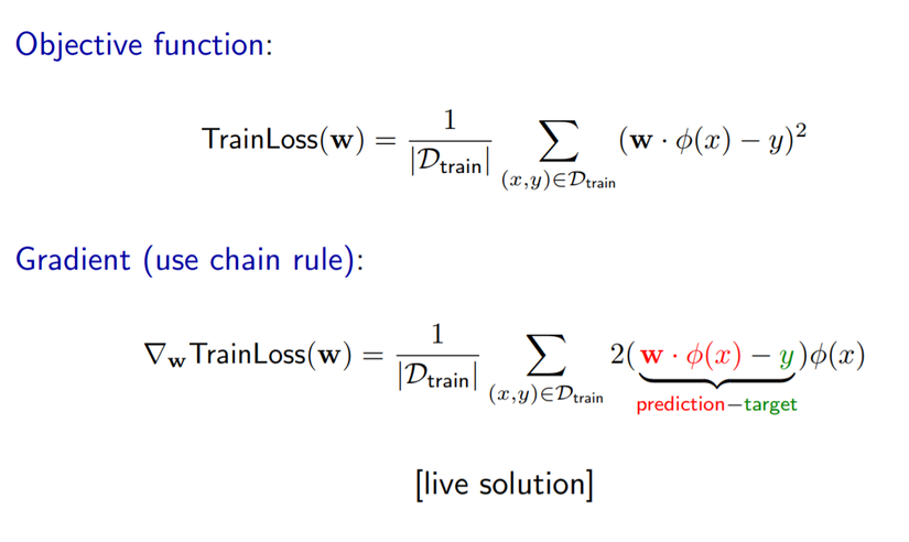All that’s left to do before we can use gradient descent is to compute the gradient of our objective function TrainLoss. The calculus can usually be done by hand; combinations of the product and chain rule suffice in most cases for the functions we care about. Note that the gradient often has a nice interpretation. For squared loss, it is the residual (prediction - target) times the feature vector $\phi(x)$. Note that for linear predictors, the gradient is always something times $\phi(x)$ because w only affects the loss through $w \cdot \phi(x)$.

Ok, We have just had interesting glance about GD algorithm. But inside, GD has some defection: each iteration requires going over all training examples — expensive when have lots of data! Recall that the training loss is a sum over the training data. If we have one million training examples (which is, by today’s standards, only a modest number), then each gradient computation requires going through those one million examples, and this must happen before we can make any progress. Can we make progress before seeing all the data? Yeah, and we find new solution: Stochastic gradient descent (SGD). Rather than looping through all the training examples to compute a single gradient and making one step, SGD loops through the examples (x, y) and updates the weights w based on each example. Each update is not as good because we’re only looking at one example rather than all the examples, but we can make many more updates this way. In practice, we often find that just performing one pass over the training examples with SGD, touching each example once, often performs comparably to taking ten passes over the data with GD. There are other variants of SGD. You can randomize the order in which you loop over the training data in each iteration, which is useful. Think about what would happen if you have all the positive examples first and the negative examples after that.

• Step size: 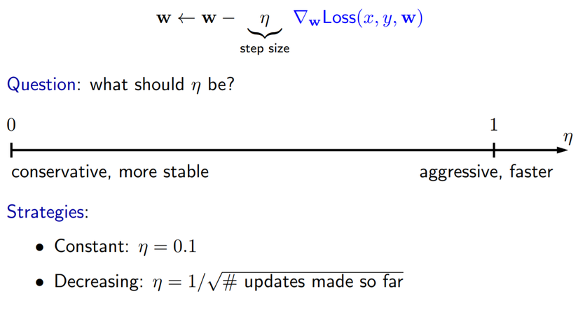One remaining issue is choosing the step size, which in practice is actually quite important, as we have seen. Generally, larger step sizes are like driving fast. You can get faster convergence, but you might also get very unstable results and crash and burn. On the other hand, with smaller step sizes, you get more stability, but you might get to your destination more slowly. A suggested form for the step size is to set the initial step size to 1 and let the step size decrease as the inverse of the square root of the number of updates we’ve taken so far. There are some nice theoretical results showing that SGD is guaranteed to converge in this case (provided all your gradients have bounded length).

Reference

https://web.stanford.edu/class/cs221/lectures/learning1.pdf