Continue with Machine Learning - Try with Multiple Algorithms
Bài đăng này đã không được cập nhật trong 8 năm
In this post, what we are trying to do is finding a way to test several algorithm then choose the best one.
DATA
The data is from https://www.kaggle.com/uciml/breast-cancer-wisconsin-data/data
Purpose
Our machine learning model here is to predict whether the case diagnosis is benign or malignant (B, M). Let's look at the data:
import numpy as np
import pandas as pd
import seaborn as sns
import matplotlib.pyplot as plt
import time

df = pd.read_csv('data.csv')
df.head()
 id diagnosis  radius_mean  texture_mean  perimeter_mean  area_mean  \
0    842302         M        17.99         10.38          122.80     1001.0
1    842517         M        20.57         17.77          132.90     1326.0
2  84300903         M        19.69         21.25          130.00     1203.0
3  84348301         M        11.42         20.38           77.58      386.1
4  84358402         M        20.29         14.34          135.10     1297.0

   smoothness_mean  compactness_mean  concavity_mean  concave points_mean  \
0          0.11840           0.27760          0.3001              0.14710
1          0.08474           0.07864          0.0869              0.07017
2          0.10960           0.15990          0.1974              0.12790
3          0.14250           0.28390          0.2414              0.10520
4          0.10030           0.13280          0.1980              0.10430

      ...       texture_worst  perimeter_worst  area_worst  smoothness_worst  \
0     ...               17.33           184.60      2019.0            0.1622
1     ...               23.41           158.80      1956.0            0.1238
2     ...               25.53           152.50      1709.0            0.1444
3     ...               26.50            98.87       567.7            0.2098
4     ...               16.67           152.20      1575.0            0.1374

   compactness_worst  concavity_worst  concave points_worst  symmetry_worst  \
0             0.6656           0.7119                0.2654          0.4601
1             0.1866           0.2416                0.1860          0.2750
2             0.4245           0.4504                0.2430          0.3613
3             0.8663           0.6869                0.2575          0.6638
4             0.2050           0.4000                0.1625          0.2364

   fractal_dimension_worst  Unnamed: 32
0                  0.11890          NaN
1                  0.08902          NaN
2                  0.08758          NaN
3                  0.17300          NaN
4                  0.07678          NaN

[5 rows x 33 columns]
Data Description
There are 10 features measured in 3 ways: mean, standard error, worst. Those 10 features are: Ten real-valued features are computed for each cell nucleus:
a) radius (mean of distances from center to points on the perimeter)
b) texture (standard deviation of gray-scale values)
c) perimeter
d) area
e) smoothness (local variation in radius lengths)
f) compactness (perimeter^2 / area - 1.0)
g) concavity (severity of concave portions of the contour)
h) concave points (number of concave portions of the contour)
i) symmetry
j) fractal dimension ("coastline approximation" - 1)
and diagnosis as malignant or benign (M,B)
Data Exploration
Let's separate the data into features and class label (what we want to predict)
y = df['diagnosis']
x = df.drop(['id', 'diagnosis', 'Unnamed: 32'], axis=1)
x.head()

#Output
radius_mean  texture_mean  perimeter_mean  area_mean  smoothness_mean  \
0        17.99         10.38          122.80     1001.0          0.11840
1        20.57         17.77          132.90     1326.0          0.08474
2        19.69         21.25          130.00     1203.0          0.10960
3        11.42         20.38           77.58      386.1          0.14250
4        20.29         14.34          135.10     1297.0          0.10030

   compactness_mean  concavity_mean  concave points_mean  symmetry_mean  \
0           0.27760          0.3001              0.14710         0.2419
1           0.07864          0.0869              0.07017         0.1812
2           0.15990          0.1974              0.12790         0.2069
3           0.28390          0.2414              0.10520         0.2597
4           0.13280          0.1980              0.10430         0.1809

   fractal_dimension_mean           ...             radius_worst  \
0                 0.07871           ...                    25.38
1                 0.05667           ...                    24.99
2                 0.05999           ...                    23.57
3                 0.09744           ...                    14.91
4                 0.05883           ...                    22.54

   texture_worst  perimeter_worst  area_worst  smoothness_worst  \
0          17.33           184.60      2019.0            0.1622
1          23.41           158.80      1956.0            0.1238
2          25.53           152.50      1709.0            0.1444
3          26.50            98.87       567.7            0.2098
4          16.67           152.20      1575.0            0.1374

   compactness_worst  concavity_worst  concave points_worst  symmetry_worst  \
0             0.6656           0.7119                0.2654          0.4601
1             0.1866           0.2416                0.1860          0.2750
2             0.4245           0.4504                0.2430          0.3613
3             0.8663           0.6869                0.2575          0.6638
4             0.2050           0.4000                0.1625          0.2364

   fractal_dimension_worst
0                  0.11890
1                  0.08902
2                  0.08758
3                  0.17300
4                  0.07678
[5 rows x 30 columns]
Let check our data distribution by checking density plot on each feature:
x.plot(kind='density', subplots=True, layout=(6,6), sharex=False, legend=False, fontsize=1)
plt.show()
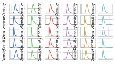 All the features quite follow a general gaussian distribution.
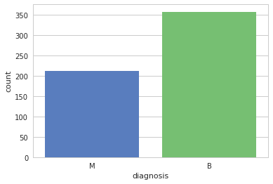
Let's check the number of case of benign and malignant
All the features quite follow a general gaussian distribution.
Let's check the number of case of benign and malignant
ax = sns.countplot(y, label="Count")
b, m = y.value_counts()
print("Number of Benign: ", b)
print("Number of Malign: ", m)
Let's check data statistics:
x.describe()

x.describe()
       radius_mean  texture_mean  perimeter_mean    area_mean  \
count   569.000000    569.000000      569.000000   569.000000
mean     14.127292     19.289649       91.969033   654.889104
std       3.524049      4.301036       24.298981   351.914129
min       6.981000      9.710000       43.790000   143.500000
25%      11.700000     16.170000       75.170000   420.300000
50%      13.370000     18.840000       86.240000   551.100000
75%      15.780000     21.800000      104.100000   782.700000
max      28.110000     39.280000      188.500000  2501.000000

       smoothness_mean  compactness_mean  concavity_mean  concave points_mean  \
count       569.000000        569.000000      569.000000           569.000000
mean          0.096360          0.104341        0.088799             0.048919
std           0.014064          0.052813        0.079720             0.038803
min           0.052630          0.019380        0.000000             0.000000
25%           0.086370          0.064920        0.029560             0.020310
50%           0.095870          0.092630        0.061540             0.033500
75%           0.105300          0.130400        0.130700             0.074000
max           0.163400          0.345400        0.426800             0.201200

       symmetry_mean  fractal_dimension_mean           ...             \
count     569.000000              569.000000           ...
mean        0.181162                0.062798           ...
std         0.027414                0.007060           ...
min         0.106000                0.049960           ...
25%         0.161900                0.057700           ...
50%         0.179200                0.061540           ...
75%         0.195700                0.066120           ...
max         0.304000                0.097440           ...

       radius_worst  texture_worst  perimeter_worst   area_worst  \
count    569.000000     569.000000       569.000000   569.000000
mean      16.269190      25.677223       107.261213   880.583128
std        4.833242       6.146258        33.602542   569.356993
min        7.930000      12.020000        50.410000   185.200000
25%       13.010000      21.080000        84.110000   515.300000
50%       14.970000      25.410000        97.660000   686.500000
75%       18.790000      29.720000       125.400000  1084.000000
max       36.040000      49.540000       251.200000  4254.000000

       smoothness_worst  compactness_worst  concavity_worst  \
count        569.000000         569.000000       569.000000
mean           0.132369           0.254265         0.272188
std            0.022832           0.157336         0.208624
min            0.071170           0.027290         0.000000
25%            0.116600           0.147200         0.114500
50%            0.131300           0.211900         0.226700
75%            0.146000           0.339100         0.382900
max            0.222600           1.058000         1.252000

       concave points_worst  symmetry_worst  fractal_dimension_worst
count            569.000000      569.000000               569.000000
mean               0.114606        0.290076                 0.083946
std                0.065732        0.061867                 0.018061
min                0.000000        0.156500                 0.055040
25%                0.064930        0.250400                 0.071460
50%                0.099930        0.282200                 0.080040
75%                0.161400        0.317900                 0.092080
max                0.291000        0.663800                 0.207500

[8 rows x 30 columns]
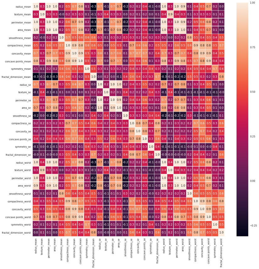
Let's check data features corrolletion:
f, ax = plt.subplots(figsize=(18,18))
sns.heatmap(x.corr(), annot=True, linewidths=0.5, fmt='.1f', ax=ax)
Training model
There are several algorithm that are good for binary classification. We will test with 5 algorithm and check out which one is the best one: Classification and Regression Trees (CART), Linear Support Vector Machines (SVM), Gaussian Naive Bayes (NB) and k-Nearest Neighbors (KNN) and RandomForestClassifier(RF).
from sklearn.model_selection import KFold, cross_val_score
from sklearn.tree import DecisionTreeClassifier
from sklearn.neighbors import KNeighborsClassifier
from sklearn.naive_bayes import GaussianNB
from sklearn.svm import SVC, LinearSVC


models = []
models.append(('CART', DecisionTreeClassifier()))
models.append(('SVM', SVC()))
models.append(('NB', GaussianNB()))
models.append(('KNN', KNeighborsClassifier()))
models.append(('LinearSVC', LinearSVC()))

num_folds = 10
results = []
names = []
kfold = KFold(n_splits=num_folds, random_state=123)
for name, model in models:
   start = time.time()
   cv_results = cross_val_score(model, x_train, y_train, cv=kfold, scoring='accuracy')
   end = time.time()
   results.append(cv_results)
   names.append(name)
   print("%s: %f (%f) (run time: %f)" % (name, cv_results.mean(), cv_results.std(), end-start))

#Output
CART: 0.919551 (0.024681) (run time: 0.069104)
SVM: 0.625769 (0.074918) (run time: 0.569782)
NB: 0.921987 (0.034719) (run time: 0.039054)
KNN: 0.901859 (0.044437) (run time: 0.046674)
RF: 0.934679 (0.032022) (run time: 0.326259)
Let's make a graph of the performance
fig = plt.figure()
fig.suptitle('Performance Comparision')
ax= fig.add_subplot(111)
plt.boxplot(results)
ax.set_xticklabels(names)
plt.show()
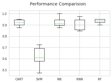
We find that the svm performance is not so good. This may be due to data not scaled yet. Let's scale before training check the performance again.
from sklearn.pipeline import Pipeline
from sklearn.preprocessing import StandardScaler
import warnings

pipelines = []

pipelines.append(('ScaledCART', Pipeline([('Scaler', StandardScaler()), ('CART', DecisionTreeClassifier())])))
pipelines.append(('ScaledSVM', Pipeline([('Scaler', StandardScaler()), ('SVM', SVC())])))
pipelines.append(('ScaledNB', Pipeline([('Scaler', StandardScaler()), ('NB', GaussianNB())])))
pipelines.append(('ScaledKNN', Pipeline([('Scaler', StandardScaler()), ('KNN', KNeighborsClassifier())])))
pipelines.append(('ScaledRF', Pipeline([('Scaler', StandardScaler()), ('RF', RandomForestClassifier())])))

results = []
names = []

with warnings.catch_warnings():
    warnings.simplefilter('ignore')
    kfold = KFold(n_splits=num_folds, random_state=123)
    for name, model in pipelines:
        start = time.time()
        cv_results = cross_val_score(model, x_train, y_train, cv=kfold, scoring='accuracy')
        end = time.time()
        results.append(cv_results)
        names.append(name)
        print("%s: %f (%f) (%f)" % (name, cv_results.mean(), cv_results.std(), end-start))

#Output
ScaledCART: 0.937179 (0.025657) (0.154313)
ScaledSVM: 0.969744 (0.027240) (0.134548)
ScaledNB: 0.937051 (0.039612) (0.058743)
ScaledKNN: 0.952115 (0.043058) (0.091208)
ScaledRF: 0.949744 (0.031627) (0.405433)

There are a lot of improvement. and SVM is the best.
Here is the crux of this post. We will use GridSearchCV from model_selection to run each important params to tune for the best params.
from sklearn.model_selection import GridSearchCV

scaler = StandardScaler().fit(x_train)
scaledX = scaler.transform(x_train)
c_values = [round(0.1 * (i+1), 1) for i in range(20)]
kernel_values = ['linear', 'poly', 'rbf', 'sigmoid']
params_grid = dict(C=c_values, kernel=kernel_values)
kfold = KFold(n_splits=num_folds, random_state=121)
grid = GridSearchCV(estimator=SVC(), param_grid=params_grid, scoring='accuracy', cv=kfold)
grid_result = grid.fit(scaledX, y_train)
print("Best: %f using %s" % (grid_result.best_score_, grid_result.best_params_))
means = grid_result.cv_results_['mean_test_score']
stds = grid_result.cv_results_['std_test_score']
params = grid_result.cv_results_['params']
for mean, std, param in zip(means, stds, params):
    print("%f (%f) with: %r" % (mean, std, param))
#Output
Best: 0.972362 using {'C': 0.1, 'kernel': 'linear'}
0.972362 (0.026491) with: {'C': 0.1, 'kernel': 'linear'}
0.841709 (0.053980) with: {'C': 0.1, 'kernel': 'poly'}
0.932161 (0.039436) with: {'C': 0.1, 'kernel': 'rbf'}
0.939698 (0.020594) with: {'C': 0.1, 'kernel': 'sigmoid'}
0.964824 (0.036358) with: {'C': 0.2, 'kernel': 'linear'}
0.861809 (0.040516) with: {'C': 0.2, 'kernel': 'poly'}
0.947236 (0.030812) with: {'C': 0.2, 'kernel': 'rbf'}
0.944724 (0.022233) with: {'C': 0.2, 'kernel': 'sigmoid'}
0.962312 (0.034665) with: {'C': 0.3, 'kernel': 'linear'}
0.866834 (0.043296) with: {'C': 0.3, 'kernel': 'poly'}
0.952261 (0.028829) with: {'C': 0.3, 'kernel': 'rbf'}
0.954774 (0.027544) with: {'C': 0.3, 'kernel': 'sigmoid'}
0.959799 (0.038022) with: {'C': 0.4, 'kernel': 'linear'}
0.869347 (0.042970) with: {'C': 0.4, 'kernel': 'poly'}
0.957286 (0.030066) with: {'C': 0.4, 'kernel': 'rbf'}
0.959799 (0.025934) with: {'C': 0.4, 'kernel': 'sigmoid'}
0.959799 (0.038022) with: {'C': 0.5, 'kernel': 'linear'}
0.871859 (0.046718) with: {'C': 0.5, 'kernel': 'poly'}
0.967337 (0.027764) with: {'C': 0.5, 'kernel': 'rbf'}
0.954774 (0.027398) with: {'C': 0.5, 'kernel': 'sigmoid'}
0.959799 (0.034560) with: {'C': 0.6, 'kernel': 'linear'}
0.876884 (0.042568) with: {'C': 0.6, 'kernel': 'poly'}
0.967337 (0.027764) with: {'C': 0.6, 'kernel': 'rbf'}
0.959799 (0.030474) with: {'C': 0.6, 'kernel': 'sigmoid'}
0.959799 (0.034560) with: {'C': 0.7, 'kernel': 'linear'}
0.884422 (0.046459) with: {'C': 0.7, 'kernel': 'poly'}
0.967337 (0.027764) with: {'C': 0.7, 'kernel': 'rbf'}
0.962312 (0.028466) with: {'C': 0.7, 'kernel': 'sigmoid'}
0.957286 (0.034271) with: {'C': 0.8, 'kernel': 'linear'}
0.894472 (0.043221) with: {'C': 0.8, 'kernel': 'poly'}
0.972362 (0.026400) with: {'C': 0.8, 'kernel': 'rbf'}
0.959799 (0.028338) with: {'C': 0.8, 'kernel': 'sigmoid'}
0.957286 (0.034271) with: {'C': 0.9, 'kernel': 'linear'}
0.896985 (0.041029) with: {'C': 0.9, 'kernel': 'poly'}
0.969849 (0.027207) with: {'C': 0.9, 'kernel': 'rbf'}
0.959799 (0.028338) with: {'C': 0.9, 'kernel': 'sigmoid'}
0.959799 (0.034560) with: {'C': 1.0, 'kernel': 'linear'}
0.902010 (0.039532) with: {'C': 1.0, 'kernel': 'poly'}
0.969849 (0.027207) with: {'C': 1.0, 'kernel': 'rbf'}
0.947236 (0.026665) with: {'C': 1.0, 'kernel': 'sigmoid'}
0.957286 (0.034271) with: {'C': 1.1, 'kernel': 'linear'}
0.902010 (0.039532) with: {'C': 1.1, 'kernel': 'poly'}
0.969849 (0.027207) with: {'C': 1.1, 'kernel': 'rbf'}
0.962312 (0.030593) with: {'C': 1.1, 'kernel': 'sigmoid'}
0.957286 (0.034271) with: {'C': 1.2, 'kernel': 'linear'}
0.902010 (0.039532) with: {'C': 1.2, 'kernel': 'poly'}
0.969849 (0.027207) with: {'C': 1.2, 'kernel': 'rbf'}
0.954774 (0.037240) with: {'C': 1.2, 'kernel': 'sigmoid'}
0.959799 (0.034560) with: {'C': 1.3, 'kernel': 'linear'}
0.902010 (0.039532) with: {'C': 1.3, 'kernel': 'poly'}
0.969849 (0.027207) with: {'C': 1.3, 'kernel': 'rbf'}
0.947236 (0.030890) with: {'C': 1.3, 'kernel': 'sigmoid'}
0.957286 (0.032387) with: {'C': 1.4, 'kernel': 'linear'}
0.902010 (0.039532) with: {'C': 1.4, 'kernel': 'poly'}
0.969849 (0.027207) with: {'C': 1.4, 'kernel': 'rbf'}
0.947236 (0.030812) with: {'C': 1.4, 'kernel': 'sigmoid'}
0.962312 (0.034665) with: {'C': 1.5, 'kernel': 'linear'}
0.907035 (0.042054) with: {'C': 1.5, 'kernel': 'poly'}
0.969849 (0.027207) with: {'C': 1.5, 'kernel': 'rbf'}
0.939698 (0.030308) with: {'C': 1.5, 'kernel': 'sigmoid'}
0.962312 (0.034665) with: {'C': 1.6, 'kernel': 'linear'}
0.907035 (0.042054) with: {'C': 1.6, 'kernel': 'poly'}
0.967337 (0.025401) with: {'C': 1.6, 'kernel': 'rbf'}
0.942211 (0.030020) with: {'C': 1.6, 'kernel': 'sigmoid'}
0.962312 (0.034665) with: {'C': 1.7, 'kernel': 'linear'}
0.907035 (0.042054) with: {'C': 1.7, 'kernel': 'poly'}
0.967337 (0.025401) with: {'C': 1.7, 'kernel': 'rbf'}
0.934673 (0.037762) with: {'C': 1.7, 'kernel': 'sigmoid'}
0.962312 (0.034665) with: {'C': 1.8, 'kernel': 'linear'}
0.907035 (0.042054) with: {'C': 1.8, 'kernel': 'poly'}
0.967337 (0.025401) with: {'C': 1.8, 'kernel': 'rbf'}
0.934673 (0.039574) with: {'C': 1.8, 'kernel': 'sigmoid'}
0.962312 (0.034665) with: {'C': 1.9, 'kernel': 'linear'}
0.907035 (0.042054) with: {'C': 1.9, 'kernel': 'poly'}
0.969849 (0.027207) with: {'C': 1.9, 'kernel': 'rbf'}
0.937186 (0.041050) with: {'C': 1.9, 'kernel': 'sigmoid'}
0.962312 (0.034665) with: {'C': 2.0, 'kernel': 'linear'}
0.909548 (0.037588) with: {'C': 2.0, 'kernel': 'poly'}
0.969849 (0.027207) with: {'C': 2.0, 'kernel': 'rbf'}
0.937186 (0.042723) with: {'C': 2.0, 'kernel': 'sigmoid'}
We found the best params. Now let's apply and test our test data.
scaler = StandardScaler().fit(x_train)
scaledx = scaler.transform(x_train)
model = SVC(C=0.1, kernel='linear')
start = time.time()
model.fit(scaledx, y_train)
end = time.time()
print("Run time: %f" % (end-start))

scaledx = scaler.transform(x_test)
y_predicted = model.predict(scaledx)

print("Accuracy score: %f" % accuracy_score(y_test, y_predicted))
print(classification_report(y_test, y_predicted))
print(confusion_matrix(y_test, y_predicted))

#Output
Run time: 0.003853
Accuracy score: 0.988304
             precision    recall  f1-score   support

          B       0.99      0.99      0.99       103
          M       0.99      0.99      0.99        68

avg / total       0.99      0.99      0.99       171

[[102   1]
 [  1  67]]
Reference
All rights reserved
