Continue with Machine Learning - Noise Detection (Classification)

Noise has pattern that we can identify. If our model is good enough to classify a specific group of noises such as gun shot, mirror broken, car horn, ..., then we can use the model in a very useful ways such as to identify crime or abnormality in a running machine by just detecting the noise.

Today we'll build a noise classifier based on the data from https://drive.google.com/drive/folders/0By0bAi7hOBAFUHVXd1JCN3MwTEU The data is the collection of noises from 10 classes. Our goal is to learn from the training data in order to identify one among those noises.

Note that we'll be using librosa libray to audio analysing. We need to convert wave form to interval of frequency. Here we change each noise into MFCCs (Mel Frequency Cepstral Coefficient), which is an array of some numbers.

All we'll be using Deep Learning algorithm to train our data with [keras](https://keras.io/) and [tensorflow](https://github.com/tensorflow/tensorflow) libraries.

We'll skip the installation process by going directly into the implementation.

Understand Data

The attributes of data are as follows: ID – Unique ID of sound excerpt Class – type of sound

Each noise is a wave file with .wav extension. Try to listen to some noises.

import IPython.display as ipd
ipd.Audio('data/Train/2022.wav')

Output

Now let's plot some waves to see their patterns.

% pylab inline
import os
import pandas as pd
import librosa
import glob
import librosa.display

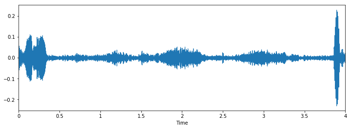
data, sampling_rate = librosa.load('data/Train/1045.wav')
plt.figure(figsize=(12, 4))
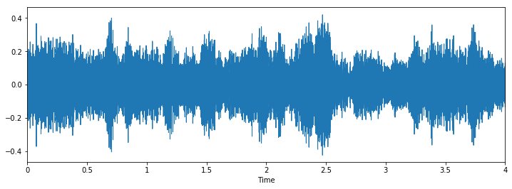
librosa.display.waveplot(data, sr=sampling_rate)

Output

Let's check some wave plots and observe its patterns. Pay attention to how the patterns of wave of the same class looks similar to each other.

import time
train = pd.read_csv('data/train.csv')
data_dir = os.getcwd() + '/data'
def load_wave():
    i = random.choice(train.index)

    audio_name = train.ID[i]
    path = os.path.join(data_dir, 'Train', str(audio_name) + '.wav')

    print('Class: ', train.Class[i])
    x, sr = librosa.load(path)

    plt.figure(figsize=(12, 4))
    librosa.display.waveplot(x, sr=sr)
    plt.show()

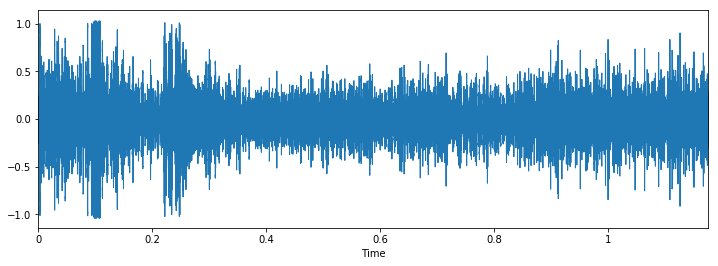
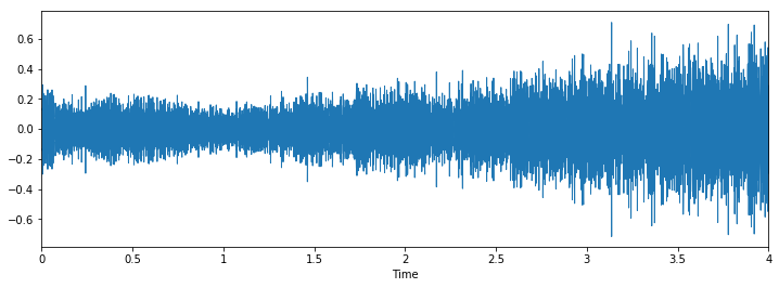
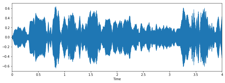
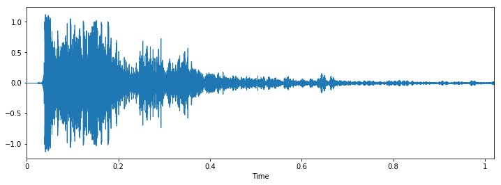
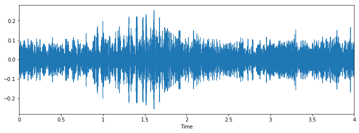
for i in range(10):
    load_wave()

Output

Class: jackhammer

Class: street_music

Class: gun_shot

Class: street_music

Class: siren

Class: engine idling

Class: children_playing

Class: gun_shot

Class: children_playing

Class: children_playing

Let's check number of values for each class:

train.Class.value_counts()

Output:

jackhammer          668
engine_idling       624
siren               607
children_playing    600
street_music        600
drilling            600
air_conditioner     600
dog_bark            600
car_horn            306
gun_shot            230
Name: Class, dtype: int64

Let's create function to convert wave to mfcc.

def parser(row):
   # function to load files and extract features
   file_name = os.path.join(os.path.abspath(data_dir), 'Train', str(row.ID) + '.wav')

   # handle exception to check if there isn't a file which is corrupted
   try:
      # here kaiser_fast is a technique used for faster extraction
      X, sample_rate = librosa.load(file_name, res_type='kaiser_fast') 
      # we extract mfcc feature from data
      mfccs = np.mean(librosa.feature.mfcc(y=X, sr=sample_rate, n_mfcc=40).T,axis=0) 
   except Exception as e:
      print("Error encountered while parsing file: ", file)
      return None, None
 
   feature = mfccs
   label = row.Class
 
   return [feature, label]

temp = train.apply(parser, axis=1)
temp.columns = ['feature', 'label']
temp.head(2)

Output

	feature	label
0	[-82.12358939071989, 139.5059159813099, -42.43...	siren
1	[-15.744005405358056, 124.1199599305049, -29.4...	street_music
2	[-123.39365145003913, 15.181946313102896, -50....	drilling
3	[-213.27878814908152, 89.32358896182456, -55.2...	siren
4	[-237.92647882472895, 135.90246127730546, 39.2...	dog_bark

[array([-82.12358939, 139.50591598, -42.43086489,  24.82786139,
       -11.62076447,  23.49708426, -12.19458986,  25.89713885,
        -9.40527728,  21.21042898,  -7.36882138,  14.25433903,
        -8.67870015,   7.75023765, -10.1241154 ,   3.2581183 ,
       -11.35261914,   2.80096779,  -7.04601346,   3.91331351,
        -2.3349743 ,   2.01242254,  -2.79394367,   4.12927394,
        -1.62076864,   4.32620082,  -1.03440959,  -1.23297714,
        -3.11085341,   0.32044827,  -1.787786  ,   0.44295495,
        -1.79164752,  -0.76361758,  -1.24246428,  -0.27664012,
         0.65718559,  -0.50237115,  -2.60428533,  -1.05346291]), array([-15.74400541, 124.11995993, -29.42888126,  39.44719325,
       -23.50191209,  16.55081468, -21.73682007,  16.533573  ,
       -16.97172924,   4.48358393, -17.38768904,   0.73712233,
       -16.28922845,   5.11214906, -10.55923116,   2.91787297,
       -10.39084829,   0.6512996 , -10.04633806,  -1.78348022,
        -6.09971424,   5.62978658,  -4.65111382,  -1.3691931 ,
        -8.24916556,  -2.36192798,  -4.79620618,  -0.50256975,
        -5.41067503,   2.07804459,   7.18600337,   8.1857473 ,
         0.76736086,   0.32726166,  -2.21366512,  -3.1068377 ,
        -5.72384895,   0.82370563,   1.7193221 ,  -0.33146235]), array([-123.39365145,   15.18194631,  -50.09332904,    7.14187248,
        -26.81703338,   -0.69250356,   -8.22307572,   13.51293887,
        -11.38205589,   19.94935211,  -11.19345959,    9.59290493,
         -8.26916969,    4.59170834,   -4.1160931 ,   -0.12661012,
         -9.26636096,   12.86464874,   -6.76813103,    0.17970622,
         -5.58614496,    6.82406367,   -7.44342262,    6.7138549 ,
          0.88696144,    7.95247415,   -7.80404736,    4.75135726,
         -5.91704383,   -0.51082848,   -2.89312164,    3.75250478,
         -4.3756492 ,    5.6246255 ,   -4.87082627,    1.88768287,
         -3.88603327,    1.57439023,   -3.9967419 ,    3.24574944]), array([-2.13278788e+02,  8.93235890e+01, -5.52561899e+01,  1.26320999e+01,
       -4.77753793e+01,  1.47029095e+01,  1.90393420e+01,  1.59744018e+01,
       -3.44622589e-01, -3.85278488e+00, -5.71352012e+00,  1.45023797e+01,
        7.35625117e+00,  2.77150926e+00, -1.21664120e+01, -7.54264413e+00,
       -1.07718201e+00, -8.32686797e+00,  1.13106934e+01,  1.30546411e+01,
       -1.24408594e+01, -1.77511089e+01,  5.21535203e-02,  2.10836481e+00,
        5.23872284e+00,  9.59365485e+00, -3.76473392e+00, -2.26955796e+00,
       -6.74119185e+00, -8.63759137e+00,  1.20566440e+01, -4.87823860e+00,
       -5.16628578e+00,  1.11927687e+00, -2.28136843e+00,  5.82950793e+00,
        1.19403556e+00,  7.46546796e+00, -1.78587829e+00, -1.50114553e+01]), array([-2.37926479e+02,  1.35902461e+02,  3.92684403e+01,  2.12402387e+01,
        9.53132848e+00,  1.38851206e+01, -3.99444661e+00,  1.24814870e+01,
       -2.60462664e+00,  6.07091558e+00,  2.23836723e+00,  4.17497228e+00,
       -1.90301314e+00,  2.30779460e+00, -2.66080009e+00, -6.64915491e-01,
        4.49824368e+00,  3.77204298e+00,  3.37126391e+00,  1.59958680e+00,
       -5.34918903e-01, -1.95140379e-01,  6.27361166e-01,  3.20973300e+00,
        1.33894133e+00,  1.04329816e-01,  9.07274421e-01, -2.27093950e+00,
       -5.29897600e-01,  2.00067343e-01,  5.41832293e-01, -3.01083238e-01,
        5.31196471e-01, -5.16148851e-01,  1.73844662e+00,  1.10963680e+00,
        2.75794074e+00,  2.15940254e+00,  6.26566792e-01,  6.92017477e-01])]

Let's convert label to dummy variable

from sklearn.preprocessing import LabelEncoder
from keras.utils import np_utils

X = np.array(temp.feature.tolist())
y = np.array(temp.label.tolist())

lb = LabelEncoder()
print(lb.fit_transform(y)[:5])
y = np_utils.to_categorical(lb.fit_transform(y))
print(y.shape)
print(y[:10])

Output

[8 9 4 8 3]
(5435, 10)
[[0. 0. 0. 0. 0. 0. 0. 0. 1. 0.]
 [0. 0. 0. 0. 0. 0. 0. 0. 0. 1.]
 [0. 0. 0. 0. 1. 0. 0. 0. 0. 0.]
 [0. 0. 0. 0. 0. 0. 0. 0. 1. 0.]
 [0. 0. 0. 1. 0. 0. 0. 0. 0. 0.]
 [0. 0. 1. 0. 0. 0. 0. 0. 0. 0.]
 [0. 0. 0. 0. 0. 0. 0. 0. 0. 1.]
 [0. 0. 0. 0. 1. 0. 0. 0. 0. 0.]
 [0. 0. 0. 0. 0. 0. 1. 0. 0. 0.]
 [0. 0. 0. 1. 0. 0. 0. 0. 0. 0.]]

Now let's build the model:

model = Sequential()

model.add(Dense(256, input_shape=(40,)))
model.add(Activation('relu'))
model.add(Dropout(0.5))

model.add(Dense(256))
model.add(Activation('relu'))
model.add(Dropout(0.5))

model.add(Dense(num_labels))
model.add(Activation('softmax'))

model.compile(loss='categorical_crossentropy', metrics=['accuracy'], optimizer='adam')

model.fit(X, y, batch_size=32, epochs=200, validation_split=0.1, shuffle=True)

Here is some last few output:

Epoch 196/200
4891/4891 [==============================] - 0s 84us/step - loss: 0.3572 - acc: 0.8779 - val_loss: 0.3988 - val_acc: 0.8989
Epoch 197/200
4891/4891 [==============================] - 0s 94us/step - loss: 0.3450 - acc: 0.8867 - val_loss: 0.3363 - val_acc: 0.9044
Epoch 198/200
4891/4891 [==============================] - 0s 84us/step - loss: 0.3603 - acc: 0.8796 - val_loss: 0.3784 - val_acc: 0.8934
Epoch 199/200
4891/4891 [==============================] - 0s 84us/step - loss: 0.3349 - acc: 0.8902 - val_loss: 0.3603 - val_acc: 0.8952
Epoch 200/200
4891/4891 [==============================] - 0s 84us/step - loss: 0.3700 - acc: 0.8814 - val_loss: 0.3686 - val_acc: 0.8952
<keras.callbacks.History at 0x7f6fb6eb6b00>

We'll see that accuracy rate is 0.8814, and validation accuracy 0.8952 the loss is around 0.37.

Pretty good result. But I think we can tune to make better result!

Conclusion

We cannot work on wave sound directly so we need to convert it to digital format first. The we use deep learning to learn from those pattern to predict the other noises.